Week 10 : Simulating Sampling Distributions for t-values

The sampling distribution is central to how we can move from t-values to p-values - yet it is one of the trickier parts of this course. The lectures and pre-lecture materials frequently deal with computer simulations to show the properties of the tests we’re using, so this week you will write your own simulation to help understand the sampling distribution!

Learning objectives for this session
	Quantitative Methods
	Sampling Distributions
	t-values
	p-values

	Data Skills
	Computing a one sample t-test in R
	Simulating data in R
	Writing loops in R

	Open Science
	Creating shareable code to demonstrate a statistical concept

1. The Dataset

TLDR: There is no data to download! we’re going to make the data ourselves.

The dataset this week is very simple - we’re going to create it ourselves using R. At this point, we know a lot about the types of questions that we can ask with t-tests and we know a lot about the data processing around it. We can check our understanding of different aspects of these statistical tests by simulating data samples that have known properties (eg mean and standard deviation) and checking if the outcome of the t-test is what we would expect.

This way we can numerically validate the tests we’re running and take a look under the hood and see what sort of processes Jamovi and R are using to compute the tests for us.

Content Info

There is a lot of code in this session - don’t be afraid to ask for help from your tutors!

2. The Challenge

Today, we’ll first introduce some concepts and functions in R to simulate a data sample and compute our own one sample t-test. With that in hand, we will set up code to run thousands of tests in one go to help us to better understand sampling distributions.

3. Code for a one sample t-test

The first thing we’ll need is to compute a t value for a one sample t-test given a dataset. We can work from this definition you’ll remember from the lectures.

\[ t = \frac{\text{The sample mean} - \text{Comparison Value}}{\text{The standard error of the mean}} \]

and

\[ \text{The standard error of the mean} = \frac{\text{The sample standard deviation}}{\sqrt{n}} \]

Let’s think about what we’ll need to do to compute our t-test. Reading through the definitions, we’ll need some basic arithmatic (+, - and /) need to use the following R functions that we have worked with in previous weeks.

Function	Definition
`mean()`	Compute the average of the numbers in a data variable
`sd()`	Compute the standard deviation of the numbers in a data variable
`sqrt()`	Compute the square root of a number

With these components, we can compute the t-value for

Check Your Understanding - Data Quiz

Questions
Hint

Match the components of the one sample t-test to the R code that computes them. We can assume that our data is in a variable named sample and the number of data points is in a variable named n. The comparison value that we want to compare our mean to is in a variable named comparison_value.

Assumption	Definition
`sample_mean =`
`sample_standard_deviation =`
`sample_standard_error =`
`t_value =`

Carefully compare the options to the equations for a t-test and R function definitions above.

Now we have our ingredients, let’s run a t-test!

Key step

Open Jamovi, install the Rj add-on and open a new Rj window before we go any further

Check Your Understanding

Take this code template and copy it across to an Rj window. Can you complete the code to compute a one-sample t-test to quantify how different the mean of sample is from the comparison_value of zero.

Copy this code into your Rj window (you can overwrite the previous code if you like), and fill in the blanks indicated by __YOUR_CODE_HERE__ (you should delete __YOUR_CODE_HERE__ and replace it with your answer).


# Number of participants
n = 25

# Generate a random sample
sample = rnorm(n, mean=0, sd=1)

# Calculate the sample mean and standard deviation
sample_mean = __YOUR_CODE_HERE__
sample_sd = __YOUR_CODE_HERE__

# Calculate the sample error of the mean 
sample_standard_error = __YOUR_CODE_HERE__

# Define comparison value
comparison_value = 0

# Compute t-value
t_value = __YOUR_CODE_HERE__

print(t_value)

All the answers are in previous sections, pay particular attention to the code examples in the previous ‘Check your understanding’ exercise.

Chat with one of your tutors if you get stuck.

The final code should look like this


# Number of participants
n = 25

# Generate a random sample
sample = rnorm(n, mean=0, sd=1)

# Calculate the sample mean and standard deviation
sample_mean = mean(sample)
sample_sd = sd(sample)

# Calculate the sample error of the mean 
sample_standard_error = sample_sd / sqrt(n)

# Define comparison value
comparison_value = 0

# Compute t-value
t_value = (sample_mean - comparison_value) / sample_standard_error

print(t_value)

Try running the code to make sure that it prints out a t-value. If you get some red text, it means something has gone wrong. Check your answers and chat with one of the tutors.

So, now we have some working code to compute our own t-values. This is going to be very useful in this session.

We have checked that the code runs, but it would be good to make sure that we’re all actually getting the same answers from the code. This is difficult at the moment as our random number generator will be producing different numbers every time (as it should!). This is normally a good thing but in a teaching setting it can make things difficult.

We can solve this issue by setting a “Random Seed” in our code. A random seed is a starting point for generating a sequence of random numbers. Think of it as the initial value that sets the stage for randomness. When you set a random seed, you ensure that the sequence of random numbers generated can be generated the same way each time. This is really critical for Reproducibility and Consistency when checking code..

In R, you can set a random seed using the set.seed() function with a number that defines the ‘initial conditions’ for the random numbers that we will generate. For example, we could use

set.seed(123)

To tell R to generate random numbers using a specific set of initial conditions. We’ll get the same sequence of numbers each time we generate a data sample. This means that if we all add the same random seed to the code, we should get the same t-value every time.

Let’s try adding the random seed to the code.

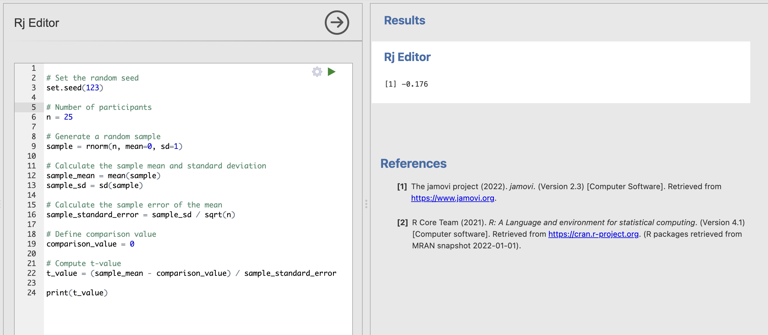
We should all get the value -0.176 as the answer. Now we can be certain that we’re all getting the right answers.

Check Your Understanding - Data Quiz

Questions

Adapt your code to compute the t-value for the following conditions. Use a random seed of 123 throughout.

A data sample of 100 participants with mean of zero and standard deviation of one with a comparison value of zero: t =
A data sample of 100 participants with mean of three and standard deviation of one with a comparison value of zero: t =
A data sample of 10 participants with mean of three and standard deviation of one with a comparison value of two: t =
A data sample of 10 participants with mean of three and standard deviation of three with a comparison value of two: t =

Key step

After completing the exercise, reset your code to the following conditions

n = 20
rnorm(n, mean=0, sd=1)
comparison_value = 0

4. Sampling distributions for one sample t-tests

Note that we’re simulating data with a mean of zero and using a comparison_value of zero as well. This is our Null Model - the t-values we get from this code are ones that might appear if there is no true effect in the data.

# My loop
num_simulations = 1000

# Create a numeric variable to store the means
t_values = numeric(num_simulations)

# Run the loop
for (i in 1:num_simulations) {
    # Number of participants
    n = 20

    # Generate a random sample
    sample = rnorm(n, mean = 0, sd = 1)

    # Calculate the sample mean and standard deviation
    sample_mean = mean(sample)
    sample_sd = sd(sample)

    # Calculate the sample error of the mean 
    sample_standard_error = sample_sd / sqrt(n)

    # Define comparison value
    comparison_value = 0

    # Compute t-value
    t_values[i] = (sample_mean - comparison_value) / sample_standard_error
}

# Plot the sampling distribution of t-values
hist(t_values, main = "Sampling Distribution of t-values", xlim=c(-4, 4),
     xlab = "Sample t-value", col = "skyblue", border = "white")

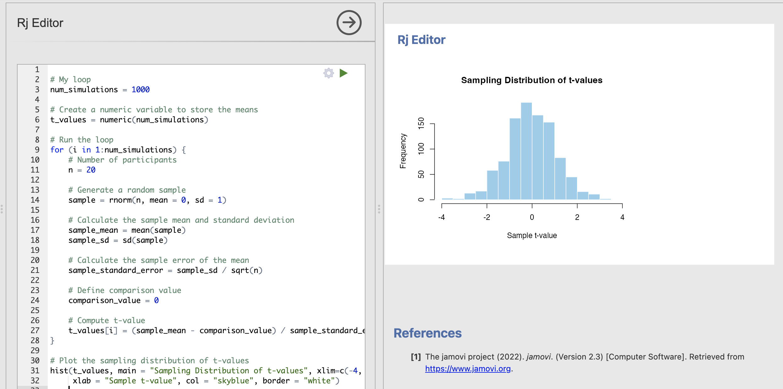
After this exercise, you can now compute the null model for a one sample t-test yourself. With this code you can run an analysis to explore how likely it is to observe different t-values when we assume the null hypothesis is true.

Think about the following questions and tweak your code to find the answers.

Data Skills - how does the sampling distribution change when we have large samples? Use n = 250 as an example.

Update your code to reduce the number of participants to 25:

    # Number of participants
    n = 250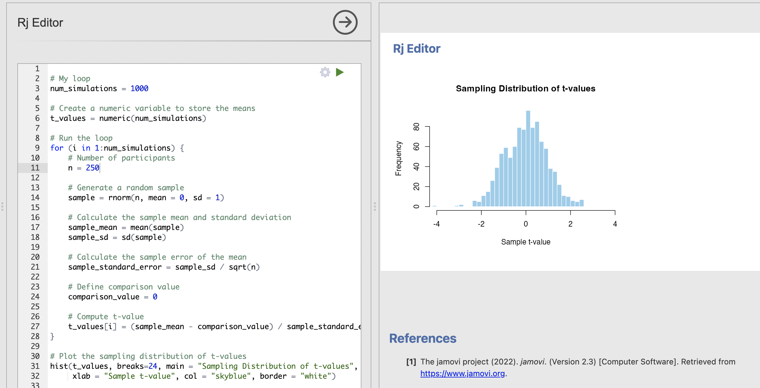

Running this a few times, you should see that the sampling distribution gets narrower compared to what we saw for n = 20. We commonly see values between -2 and 2 but almost never see values of -3 or +3.

Data Skills - how does the sampling distribution change when we have very small samples? Use n = 4 as an example.

Update your code to reduce the number of participants to 5:

    # Number of participants
    n = 4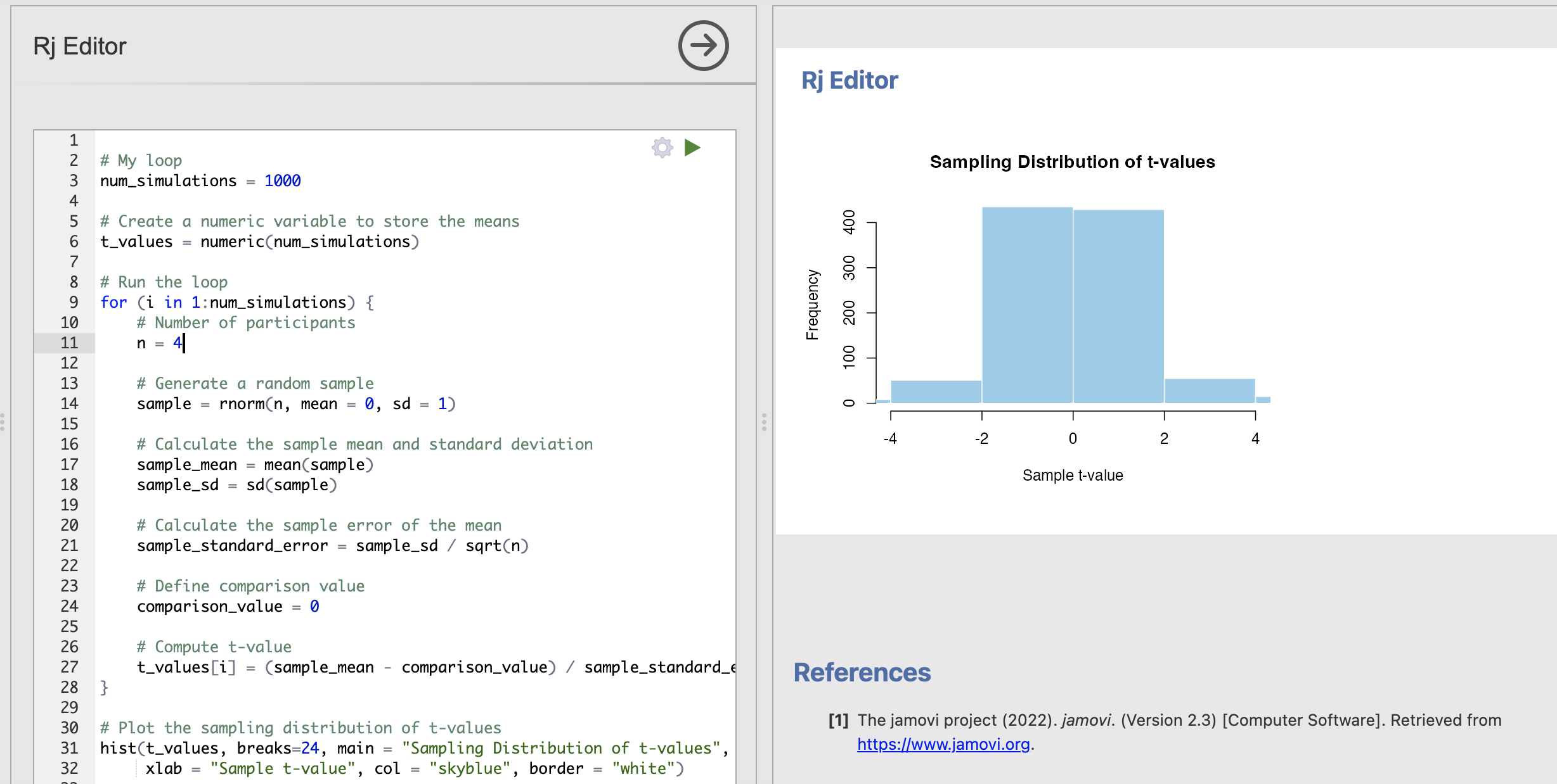

Running this a few times, you should see that the sampling distribution gets broader than for smaller samples. We see more values close to 4 and -4 than we did with a dataset of 20 or 250.

In all of these analyses we are absolutely assuming that the null hypothesis of no difference is true. With this assumptions, our sampling distribution shows that we get more extreme t-values (around +/- 4) by chance when working with smaller data samples. By contrast for larger data samples these same values occur extremely rarely.

When data are perfectly normally distributed (parametric assumptions are met), Jamovi and R can compute these null distributions for us using a shortcut without simulating lots of data samples but the result is the same.

5. The null model

We introduced the idea of a null model in the lectures. This is a model of what the outcome of our statistics would look like if the data have a random and unbiased structure. The null model is closely linked to the null hypothesis - it describes the probability to observing a particular outcome from our statistics under the assumption that the null hypothesis is true.

The sampling distributions we have computed above are exactly null models. We have

Defined population parameters in which we know for sure that the mean is zero
Sampled data observations from that population
Computed the one sample t-test between the data sample and zero
Stored the t-value for every single resampling
Visualised the distribution of t-values with a histrogram

The critical point here is that the null distribution is very stable. We can make confident predictions about what the null distribution of t-values will look like when there is no effect. Let’s try some examples:

Check Your Understanding - Data Quiz

Questions
Hint

How does the distribution of t-values change when we make these changes? Importantly, we know that there is no effect (no difference between the population mean and the comparison value) in all of these examples.

Remember that we are using random sampling so run each example a few times to get a sense of the result.

How does the t-value distribution change when:

…we increase the standard deviation of the population parameters?
…we decrease the standard deviation of the population parameters?
…we change the mean and comparison value (keeping both values the same)?

Read through your code carefully to find the component that you should change.

Talk with your tutor if you’re stuck.

(We’ll look at changing the means more in a later section…)

So, the null model for our t-tests is the sampling distribution of t-values when we know there is no effect. Critically this null module is super stable! We can make a lot of changes to the population parameters and precise values being compared and the distribution remains largely the same. We saw in the previous section that sample size can change the tails of the distribution a bit, but most of the rest doesn’t make a big difference.

This is a critical point that enables us to complete our statistical assessment. Now that we can be really confident about the probability of observing a particular t-value under the assumption that there is no effect - we’re ready to compute a p-value for our hypothesis test.

6. Computing a p-value

Remember the definition of the p-value from the lectures, this is a bit fiddely but will hopefully make some more sense now that you’re more familiar with the null model. Take a look at the lecture materials from week 5 if you need a refresher.

The p-value tells us the probability of obtaining test results at least as extreme as the result actually observed, under the assumption that the null hypothesis is correct.

We now have all the ingredients to compute this value. We need

A null model distribution telling us how likely we are to observe particular t-values when we assume the null hypothesis is correct
The t-value from a particular data sample
A statistical significance threshold

To conduct a hypothesis test, we need to compare an individual t-value from a test to the null distribution of t-value that we have just computed. Remember that the null distrbution is very stable - if we know the sample size then we can use the same null distribution for any t-test!

Let’s put this into practice.

Key step

Before going any further, reset your code to the following conditions

n = 20
rnorm(n, mean=0, sd=1)
comparison_value = 0

We can visualise where one single t-value is on a histogram by using a convenient R function named abline() which can be used to plot straight lines on a figure. We can use abline() as follows:

abline(v = 1, col = "red", lwd = 2)

This has specified three input arguments.

Input	Description
`v`	A value at which to plot a Vertical line
`col`	Optional input to choose a colour
`lwd`	Optional input to specify the width of the line `lwd=1` is a thin line and `lwd=5` would be very thick.

We can add this to the bottom of our code to see where a t-value of 1 (defined by v=1 in the function) would appear on the null distribution. Try changing the value of v a few times to see the difference.

Jamovi Issue

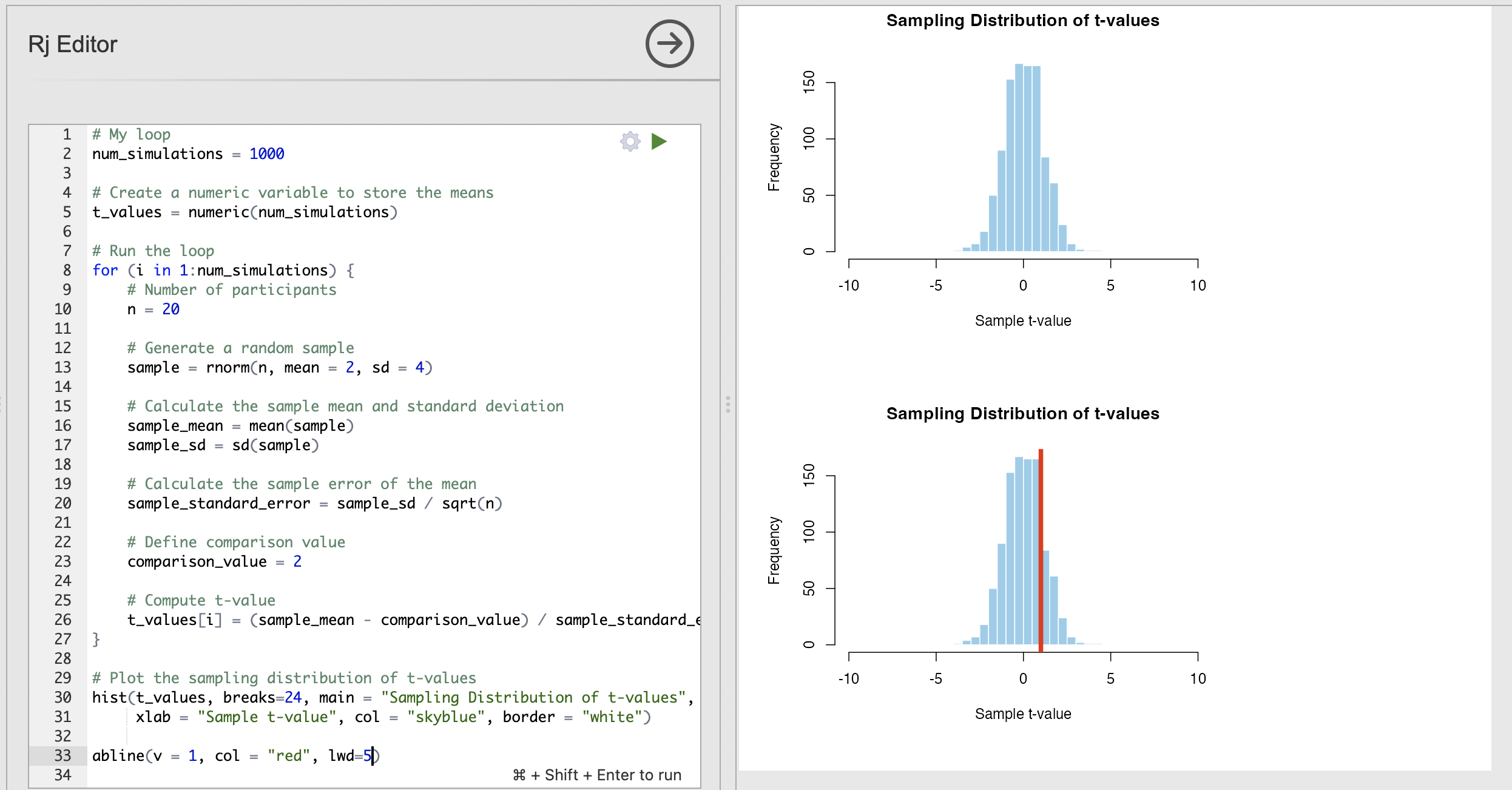
It is likely that Jamovi will present two plots when you run this code rather than one. If this happens you will have one plot for the histogram and a second for the same histogram with the vertical line (example in the image above).

I’m not sure why this happens but it is a mostly harmless quirk of Rj - please ignore the first plot!

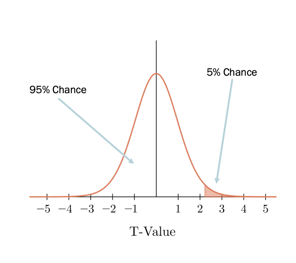
The p-value describes the probabilty of observing a t-value as least as large as the one from our test. This is equivalent to ‘cutting’ the null distribution at the specific t-value and calculating how likely it is to see a result that is more extreme than the point of the cut.

For example, from the lecture notes, here we have a parametric null distribution of t-values (parametric meaning that it wasn’t computed from simulations) that is cut at a position that means we have a 5% chance of observing a value at least as extreme as the cut.

We can do the same to compute the probability of observing a value to the left or to the right of the vertical line we’ve added to our plot. We can use some simple maths to compute exactly this value

# Compute the percentile of the value 1
observed_value = 1
percentile = sum(t_values >= observed_value) / length(t_values)
print(percentile)

This code does the following steps:

sum(t_values >= observed_t_value) counts how many values in the data are larger than or equal to the specified value.
length(t_values) gives the total number of values in the data.
Dividing the count by the total number of values converts the result into a decimal indicating the proportion of values in t_values that are larger than or equal to observed_t_value.

The final value of percentile is then our p-value, which exactly matches the definition from the lecture.

The p-value tells us the probability of obtaining test results at least as extreme as the result actually observed, under the assumption that the null hypothesis is correct.

Let’s put all of this together in our code.

set.seed(123)

# My loop
num_simulations = 1000

# Create a numeric variable to store the means
t_values = numeric(num_simulations)

# Run the loop
for (i in 1:num_simulations) {
    # Number of participants
    n = 20

    # Generate a random sample
    sample = rnorm(n, mean = 2, sd = 4)

    # Calculate the sample mean and standard deviation
    sample_mean = mean(sample)
    sample_sd = sd(sample)

    # Calculate the sample error of the mean 
    sample_standard_error = sample_sd / sqrt(n)

    # Define comparison value
    comparison_value = 2

    # Compute t-value
    t_values[i] = (sample_mean - comparison_value) / sample_standard_error
}

observed_t_value = 2.3
percentile <- sum(t_values >= observed_t_value) / length(t_values)

print('My t-value')
print(observed_t_value)
print('My p-value')
print(percentile)


# Plot the sampling distribution of t-values
hist(t_values, breaks=24, main = "Sampling Distribution of t-values", xlim=c(-10, 10),
     xlab = "Sample t-value", col = "skyblue", border = "white")
     
abline(v = observed_t_value, col = "red", lwd=5)

Here, we’ve added some code to specify a t-value from some data that we need to compute a p-value for (observed_t_value = 2.3), we compute and print the associated p-value and create the histogram with a red line indicating the position of observed_t_value.

The result should look like this (ignoring this odd double plot…)

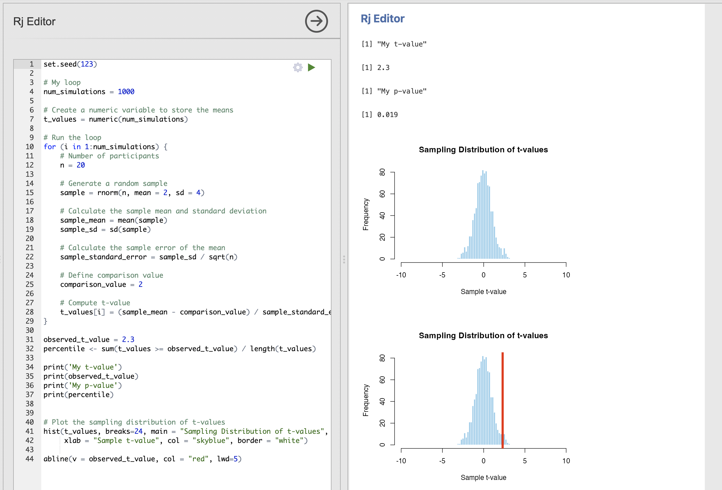
If you have set.seed(123) at the top of your script you should have exactly the same values that I do.

The results are telling us that we have a p-value of 0.019. This is less than our conventional threshold of 0.05 so we would consider a t-value of 2.3 to be statistically significant.

Our code is only checking the right sided tail of the null distribution. This is ok as we can assume that the null distribution of t-values is symmetrical. This is a key point that means we can simplify some things.

This is a One-Tailed test, as we are only considering one side of the distribution in our p-value calculation. A two-tailed test is simple though, simply divide the p-value by 2 as the lower tail should have an identical shape. For example if our code says that a result has a one-tailed p-value of 0.08 then the two-tailed p-value is 0.04.
Our code is only checking the high end of the distribution (values to the right of the red line). p-value for a negative t-value is simple to compute though. It is just one with the computed p-value subtracted from it. eg if we have a t-value of -1, our code will say that 0.837 (or 83.7%) of the null values are larger - we can simply subtract it from one to get the correct p-value 1 - 0.837 = 0.163.

Check Your Understanding - Data Quiz

What is the p-value for the following values of observed_t_value? Make sure you have set.seed(123) set at the top of your script or the values will differ from mine!

`observed_t_value`	Tail of test	p-value
1	One-Tailed
3	One-Tailed
2.5	Two-Tailed
-1.4	One-Tailed
-0.5	Two-Tailed

Carefully read the key points from the bullet points above about converting values. Talk with your tutor if you get stuck.

`observed_t_value`	Tail of test	p-value	Explanation
1	One-Tailed	`0.151`	Take the result directly from the script
3	One-Tailed	`0.001`	Take the result directly from the script
2.5	Two-Tailed	`0.01 / 2 = 0.005`	Divide the result from the script by 2.
-1.4	One-Tailed	`1 - 0.915 = 0.085`	Subtract the result from 1
-0.5	Two-Tailed	`(1 - 0.685) / 2 = 0.1575`	Subtract the result from 1 AND then divide by 2

Key step

Take a moment to feel good about yourself if you have made it this far. These are not straightforward concepts and take time to get used to. Seriously well done!

If you’re here but still finding it tough, don’t worry - speak with one of your workshop tutors and they can help to explain things to you.

7. OPTIONAL: Why do we test the null hypothesis?

Finally, let’s consider why we test against the null distribution of no effect. This is a weird concept but is fairly straightforward to see why we have to do it based onfrom the code we have written so far.

We can absolutely compute a sampling distribution for a case where there is a real difference between the mean and the comparison value. For example, this code simulates data with a mean of 1 and compares that to a comparison value of 0. Note that the rnorm() function inputs have changed.

set.seed(123)

# My loop
num_simulations = 1000

# Create a numeric variable to store the means
t_values = numeric(num_simulations)

# Run the loop
for (i in 1:num_simulations) {
    # Number of participants
    n = 20

    # Generate a random sample
    sample = rnorm(n, mean = 1, sd = 1)

    # Calculate the sample mean and standard deviation
    sample_mean = mean(sample)
    sample_sd = sd(sample)

    # Calculate the sample error of the mean 
    sample_standard_error = sample_sd / sqrt(n)

    # Define comparison value
    comparison_value = 0

    # Compute t-value
    t_values[i] = (sample_mean - comparison_value) / sample_standard_error
}

observed_t_value = 2.3
percentile <- sum(t_values >= observed_t_value) / length(t_values)

print('My t-value')
print(observed_t_value)
print('My p-value')
print(percentile)

# Plot the sampling distribution of t-values
hist(t_values, breaks=24, main = "Sampling Distribution of t-values", xlim=c(-10, 10),
     xlab = "Sample t-value", col = "skyblue", border = "white")
     
abline(v = observed_t_value, col = "red", lwd=5)

The result is a sampling distribution which is not centred around mean.

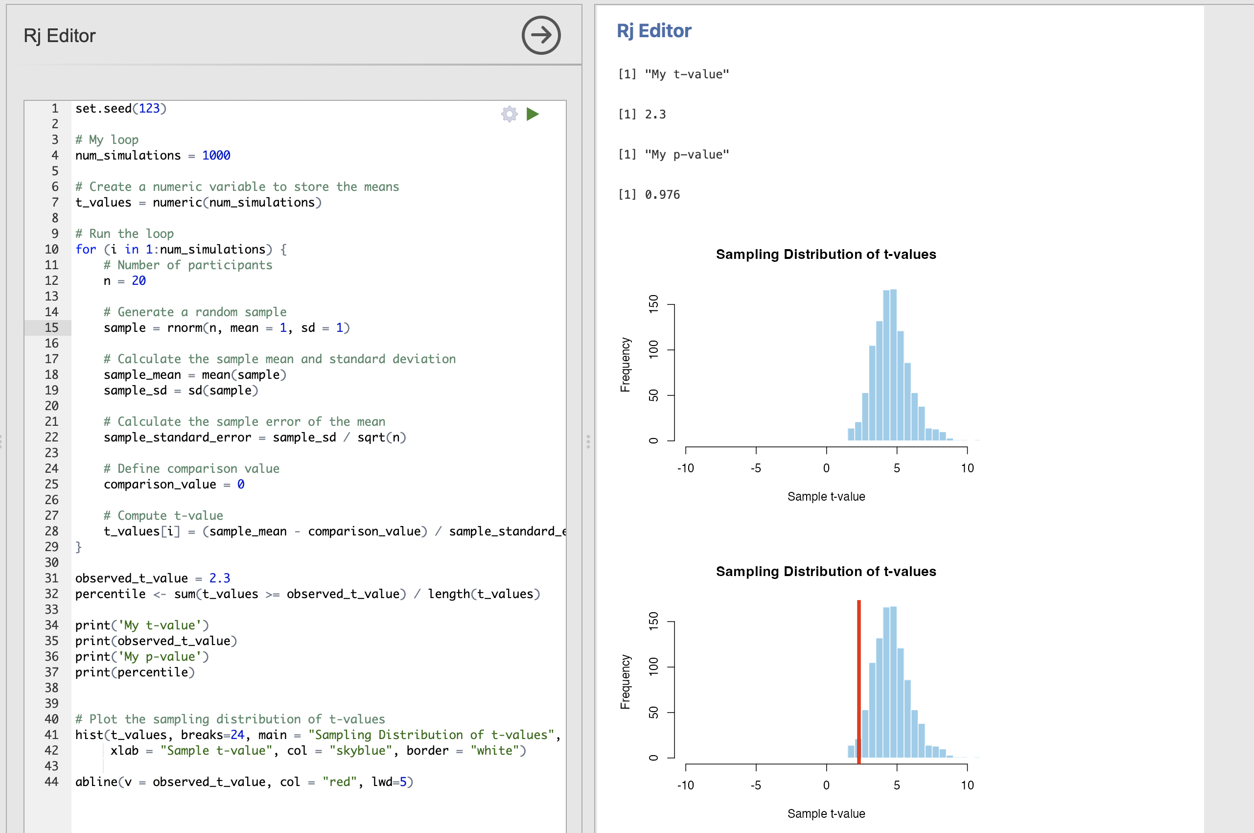
This distribution tells us that with 20 participants, a mean of 1 and a standard deviation of 1 - we are mostly likely to get a t-value of 5 but that t-value could be as small as 2 or as large as 9 for extreme data samples.

This is very useful, but the issue that is we have had to assume what the real effect is. We get radically different sampling distributions if we change that effect around. Take a look at these examples.

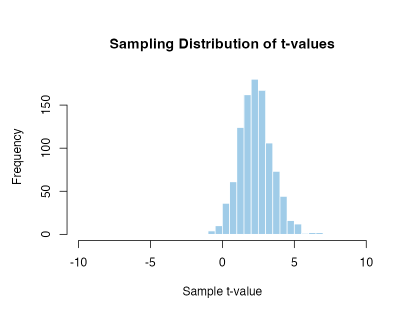
Mean of 0.5 and standard deviation of 1 with 20 participants compared to zero.

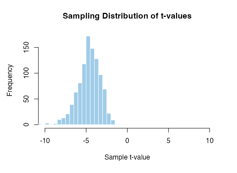
Mean of -1 and standard deviation of 1 with 20 participants compared to zero.

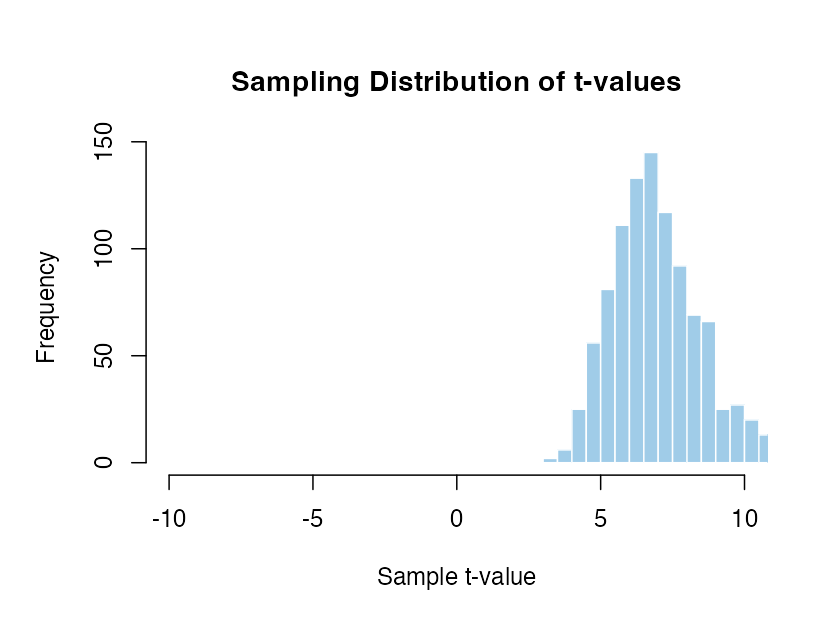
Mean of 1.5 and standard deviation of 1 with 20 participants compared to zero.

The distributions move around so much that the percentile value of the same t-value would be completely incomparable. A t-value of 5 is hugely unlikey in some cases and very frequent in others. If we have to assume that there is a specific effect the result would be extremely senstive to exactly what that assumption is. In contrast there is only one distribution to work with if we assume there is no effect.

There are an infinite number of possible sampling distributions when there is a real effect! It isn’t possible to know which distribution we should be comparing with without making some massive assumptions about the exact size, variability and direction of effect that we expect to see. This simply isn’t possible in practice.

In contrast, the null case is very closely controlled and easier to work with. The interpretation is trickier but rejecting the null hypothesis is a tractable problem that we can do a good job of solving.

8. Summary

It is worth repeating - well done for completing this session. It can be hard work developing the code to explore sampling distributions, t-values and p-values but it is a fantastic way to gain a more intuitive understanding of how and why we do things the way we do.

Week 10 : Simulating Sampling Distributions for t-values

1. The Dataset

2. The Challenge

3. Code for a one sample t-test

4. Sampling distributions for one sample t-tests

5. The null model

6. Computing a p-value

7. OPTIONAL: Why do we test the null hypothesis?

Mean of 0.5 and standard deviation of 1 with 20 participants compared to zero.

Mean of -1 and standard deviation of 1 with 20 participants compared to zero.

Mean of 1.5 and standard deviation of 1 with 20 participants compared to zero.

8. Summary

References