Week 5 : p-values and effect sizes

This week we will explore how to use the jmv package in R to test hypotheses about a dataset using t-tests and to compute effect sizes corresponding to those tests. We will use those effect sizes to help interpret the sensitivity and power of our experiments.

Learning objectives for this session
	Quantitative Methods
	Cohen’s d effect size
	Power analysis

	Data Skills
	Use `mutate()` in R to compute a new variable
	Compute t-tests using the `jmv` R package
	Run a power analysis in Rj

	Open Science
	Understand and validate code written by someone else
	Use power analysis to recommend a sample size for a replication

1. The Dataset

Dataset

Please note, this is the same dataset as we used in week 4 - but make sure that you load in the rmb-week-3_lecture-quiz-data_ai-faces-2026.omv file from this week and NOT the week 4 file. It contains a small fix that we need for this week.

We’ll be working with the dataset we collected after the break during the lecture in Week 3. This is a partial replication of a study published in the journal Psychological Science (Miller et al. 2023). The original paper found the following results summarised in the abstract.

Recent evidence shows that AI-generated faces are now indistinguishable from human faces. However, algorithms are trained disproportionately on White faces, and thus White AI faces may appear especially realistic. In Experiment 1 (N = 124 adults), alongside our reanalysis of previously published data, we showed that White AI faces are judged as human more often than actual human faces—a phenomenon we term AI hyperrealism. Paradoxically, people who made the most errors in this task were the most confident (a Dunning-Kruger effect). In Experiment 2 (N = 610 adults), we used face-space theory and participant qualitative reports to identify key facial attributes that distinguish AI from human faces but were misinterpreted by participants, leading to AI hyperrealism. However, the attributes permitted high accuracy using machine learning. These findings illustrate how psychological theory can inform understanding of AI outputs and provide direction for debiasing AI algorithms, thereby promoting the ethical use of AI.

We ran a quiz that students in the lecture could join on their phones/laptops. There were two parts to the quiz:

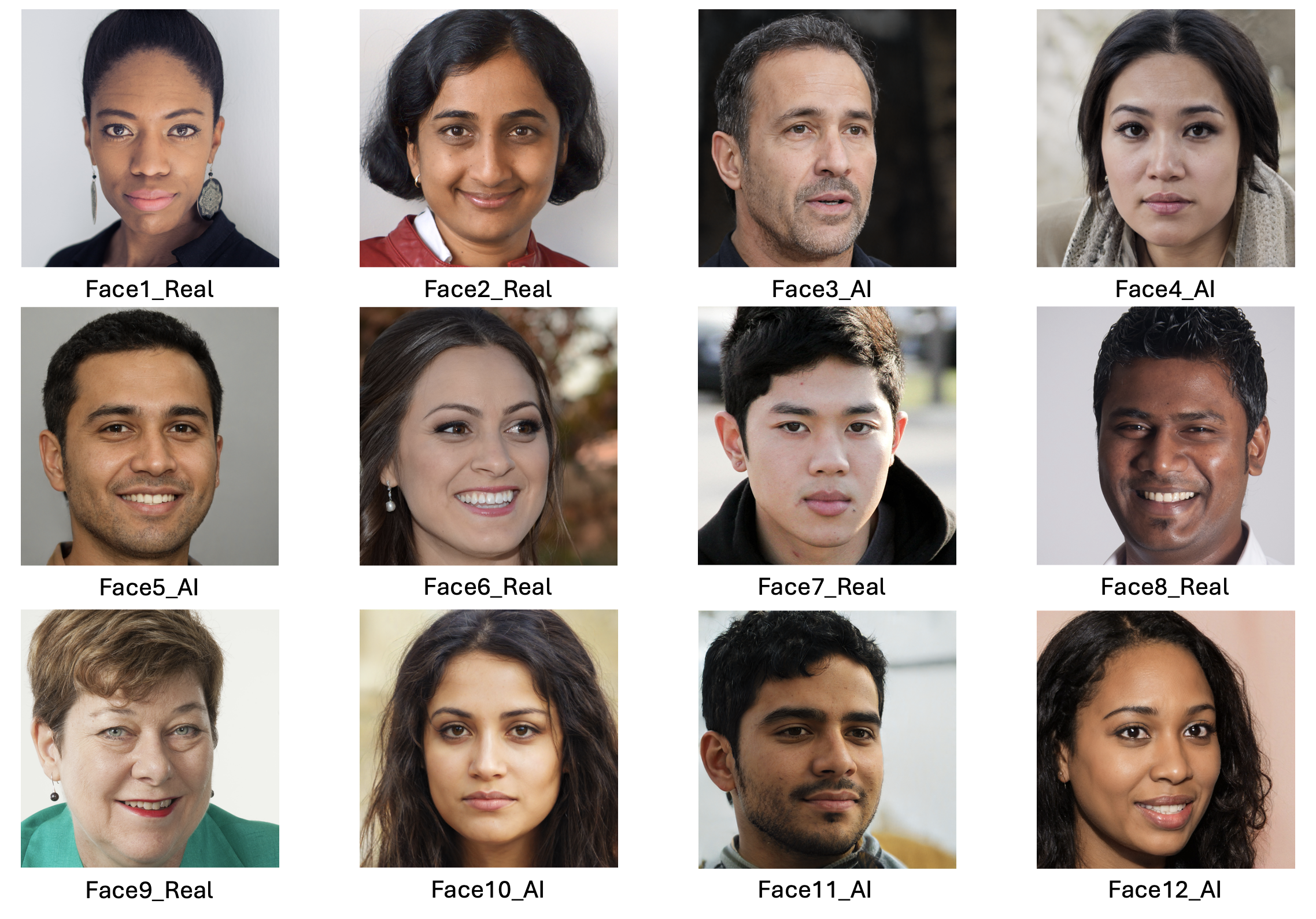
The faces section included 12 faces that were either photographs or real people or AI generated images of people. The stimuli were taked from the materials released by (Miller et al. 2023) on the Open Science Framework. Responses were either ‘Real person’ or ‘AI generated’.

The confidence section asked participants to rate their confidence in their ability to do the following three things.

Distinguish real photos of people from AI generated images (Experimental condition)
Distinguish photos of happy people from photos of sad people (Emotional control condition)
Distinguish photos of people you used to know in primary school from strangers (Memory control condition)

Scores were recorded on a scale from 1 (Completely confidence) to 10 (Not at all confident). The confidence section was repeated before and after the faces section to see if participants confidence changed as a result of doing the AI faces task

2. The Challenge

This week we will explore some factors that influence t-stats and p-values whilst introducing the concept of loops in R. We will finish by using effect sizes to compute a power analysis.

3. Compute new variables with `mutate()`

Last week, we used Jamovi to create several new variables that allowed us to run our analyses. We can do the same in a more transparent and reproducible way using R code.

We need to create both our proportion of correct faces across the 12 stimuli in one variable and a grouping variable which indicates whether each participant was confident in their ability to tell the difference between AI faces and real faces.

We can do both with the mutate() from the dplyr library, this provides functionality that lets us create, modify, and delete columns within a dataset. Take a look at the official documentation for mutate for more information.

When computing a new varaible with mutate() we three pieces of information.

The dataset to work on
The name of the new variable to be created
The definition of how to compute the new variable for existing variables.

Compute the grouping variable

Let’s start with our grouping variable. Our three pieces of information are

The dataset to work on - is data, which refers to the original datasheet loaded into Jamovi
The name of the new variable - is ConfidentBefore, the same as we used last week
The definition - is AIConfidenceBefore<4, again the same as we used last week

We can combine these into a single line to create the variable. Note that we save the result into a new variable named my_data, we’ll use this from now on to avoid confusion with the original datasheet.

library(dplyr)
my_data <- mutate(data, ConfidentBefore = AIConfidenceBefore<4)

We can check that this has done what we expected by running head to see the first few rows of the dataset.

head(my_data)

The result should look like this:

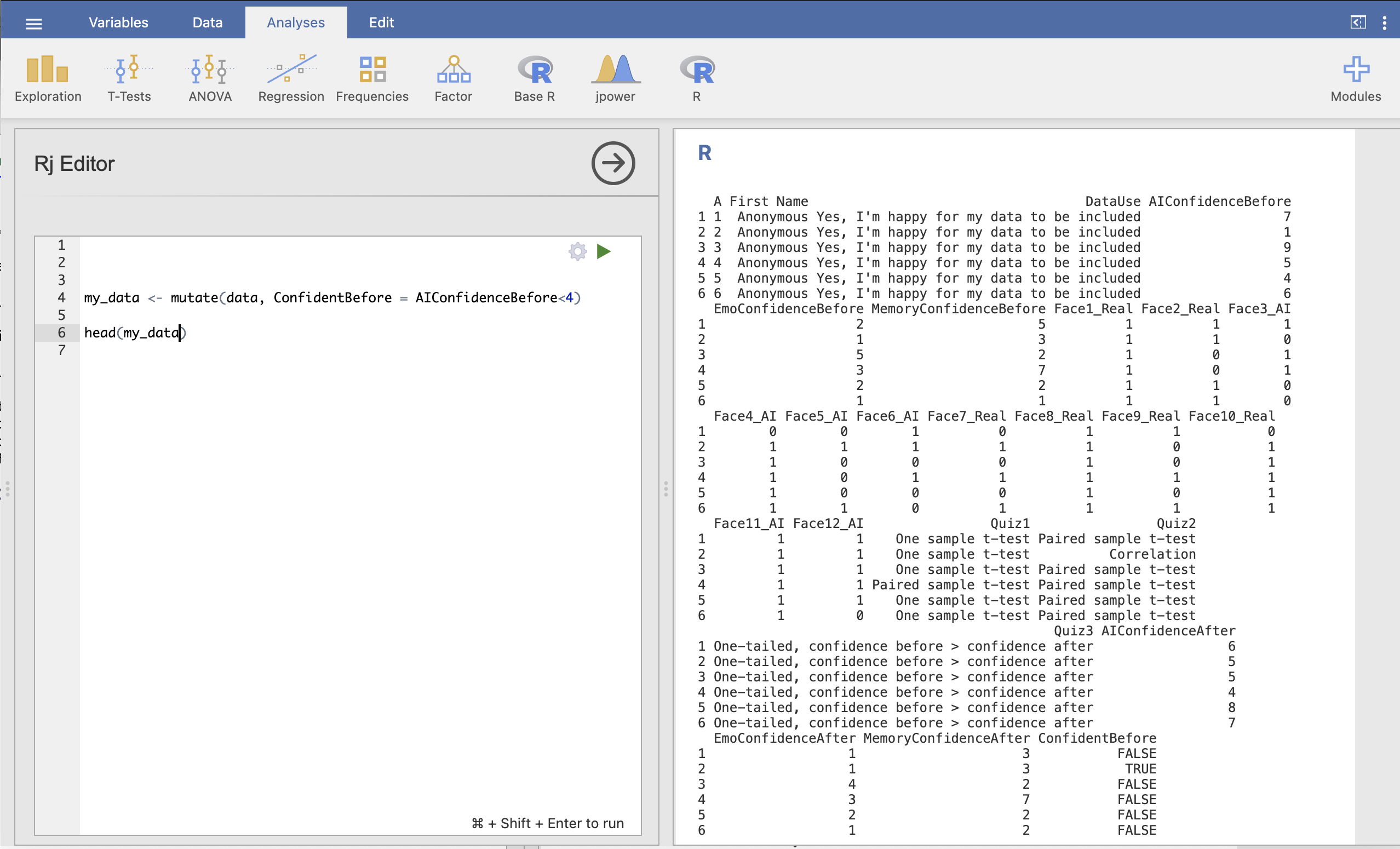
We can see on in the results on the right hand side that the additional colume ConfidentBefore now appears with TRUE and FALSE values for each participant.

Compute the proportion of correct responses

Let’s do the same for total proportion of correctly identified faces. We can use the same principle as we used for the grouping variable and use mutate() along with the variable definition and name to create our new column.

This definition is pretty long as we have 12 different faces to work with! You can copy the whole line using the copy icon in the right hand side of the code box. Take a moment to look through and understand each part: which part is the Dataset, the Name and the Definition?

my_data <- mutate(my_data, PropFacesCorrect = (Face1_Real + Face2_Real + Face3_AI + Face4_AI + Face5_AI + Face6_AI + Face7_Real + Face8_Real + Face9_Real + Face10_Real + Face11_AI + Face12_AI) / 12)

and validate the overall result using head() to make sure that my_data now has the column we expected.

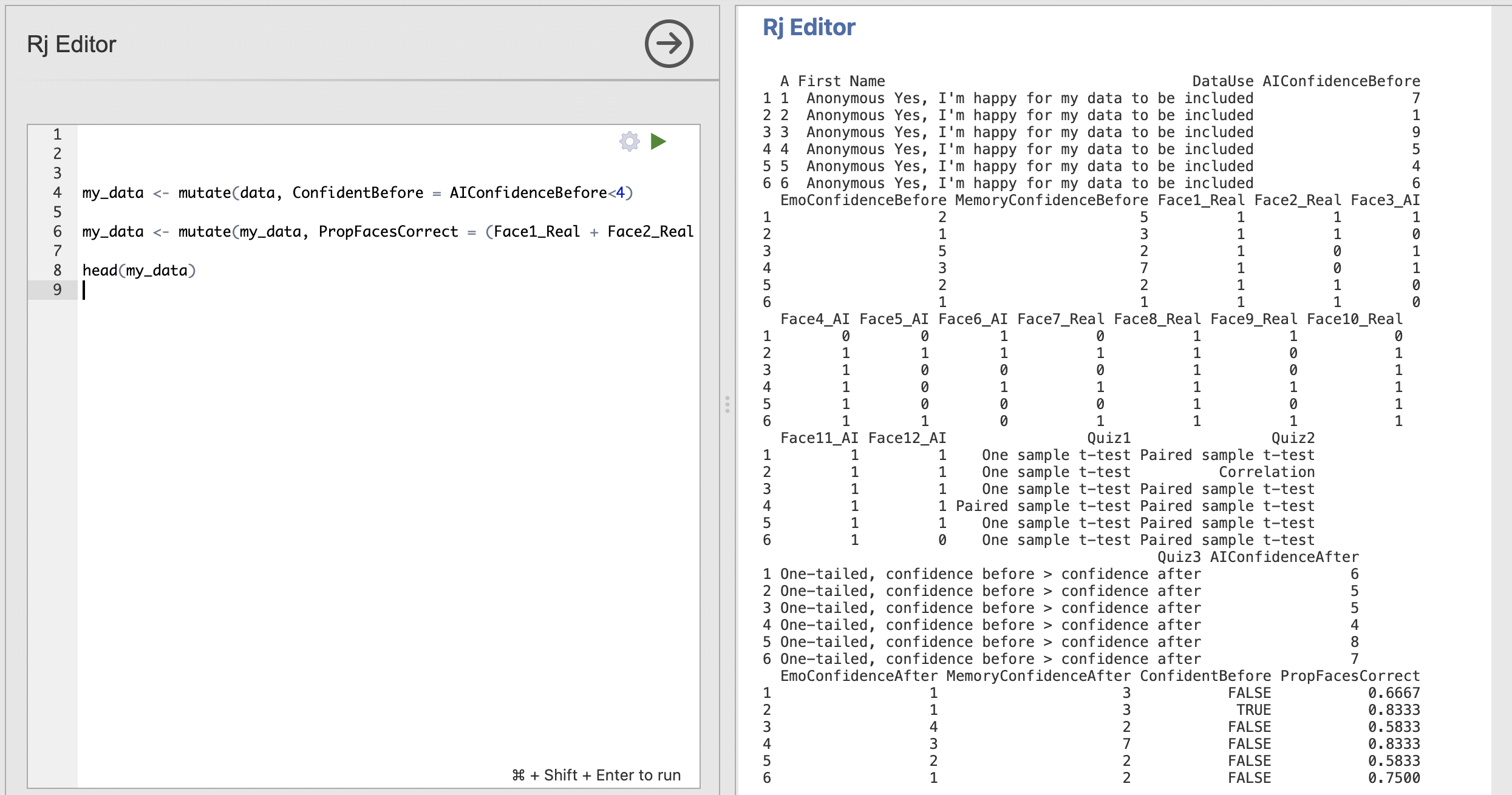
The final column of the dataset is now PropFacesCorrect and contains the proportion of face trials that participant got right.

Check Your Understanding

Can you compute variables containing the proportion of correct responses for photos of real people and AI generated faces separately?

Store the results in PropRealCorrectFaces for real faces and PropAICorrectFaces for AI generated faces.

We can use the code we wrote to compute the proportion of correct responses for all faces as a starting point.

Think about how you could modify this line to compute the result for either real or AI faces on their own? What would you need to change in the code?

The following code will compute the variables

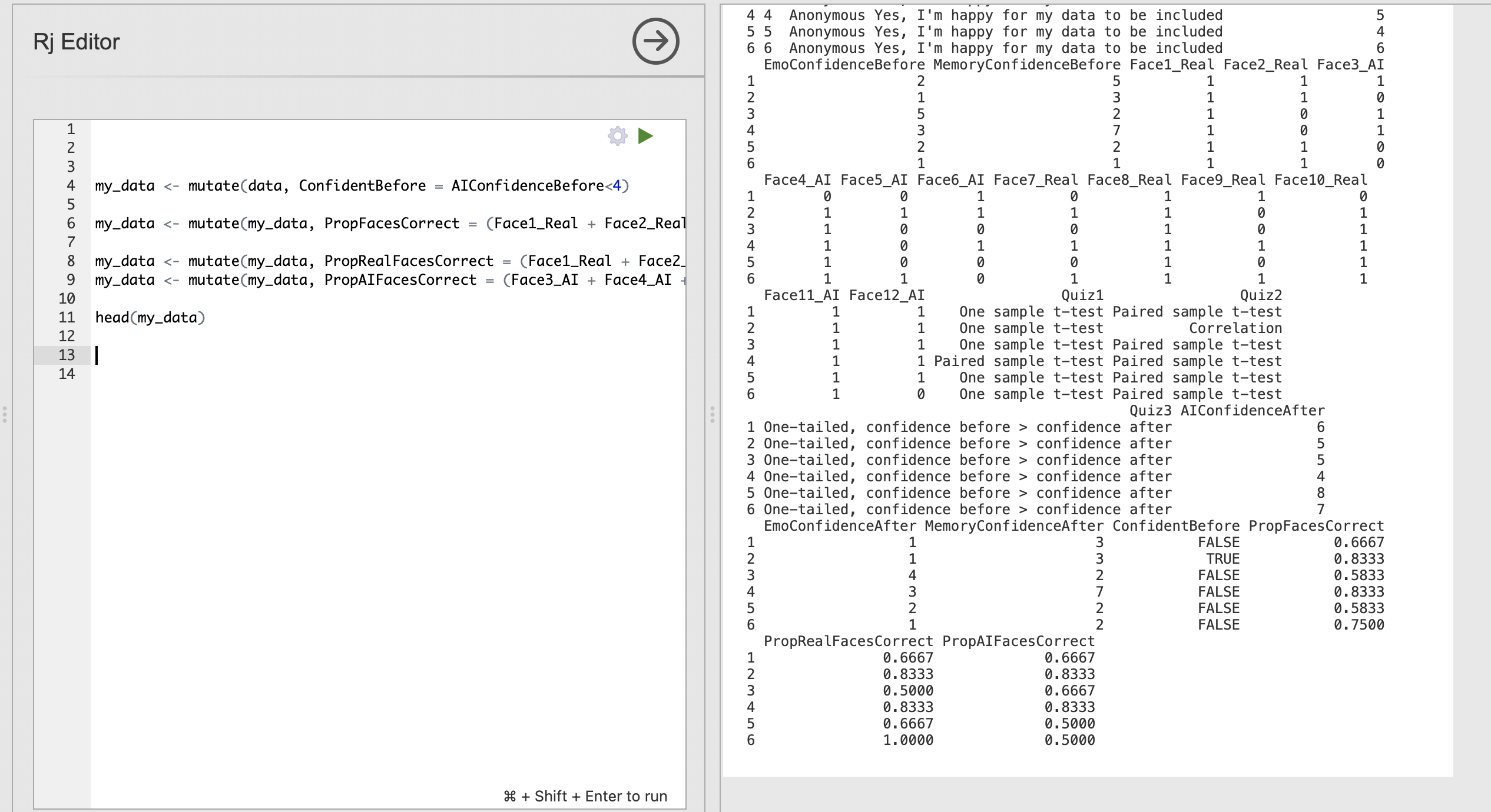
my_data <- mutate(my_data, PropRealFacesCorrect = (Face1_Real + Face2_Real + Face7_Real + Face8_Real + Face9_Real + Face10_Real) / 6)
my_data <- mutate(my_data, PropAIFacesCorrect = (Face3_AI + Face4_AI + Face5_AI + Face6_AI + Face11_AI + Face12_AI) / 6)

We’ve separated out the columns to sum all the real or AI faces together and changed the division to divide the results by 6 rather than 12.

Checking the results with head() should produce the following outputs with four additional columns!

4. Compute a t-test using R

We have the ingredients for our hypothesis test. Let’s use R to explore the following hypothesis (Hypothesis 2 from week 4).

Confident people are better at distinguishing AI faces from real faces

We can compute this test using the following code that calls ttestIS() - this is the function that computes independent samples t-tests. Read more about it on the ttestIS documentation page.

You can click the numbers by the definitions at the bottom to highlight the corresponding part of the code.

1jmv::ttestIS(
2    formula = PropFacesCorrect ~ ConfidentBefore,
3    data = my_data,
4    effectSize = TRUE)

1: jmv::ttestIS is the name of the R function that Jamovi uses to compute independent samples t-tests
2: This tells ttestIS the formula that defines the test we want to run.
3: This tells ttestIS which dataset we want to analyse
4: This adds an additional effect size computation to the results

Most of this will be familiar from previous weeks, but let’s think about the formula in a little more detail.

In R, the tilde (~) is used in formula definitions to specify the relationship between variables, particularly in statistical modeling and data analysis. Here, the tilde separates the dependent variable (response) from the independent variables (predictors). In our example, PropFacesCorrect is the dependent variable and ConfidentBefore is our independent variable (grouping variable) - so this formula

PropFacesCorrect ~ ConfidentBefore

is essentially telling ttestIS() to “Compute the ttest on PropFacesCorrect using ConfidentBefore as our groups”.

We can now run all our code to get the results of the ttest - the code clearly tells the reader how all the relevant variables were computed and what hypothesis test has been run all in one screen.

Check Your Understanding

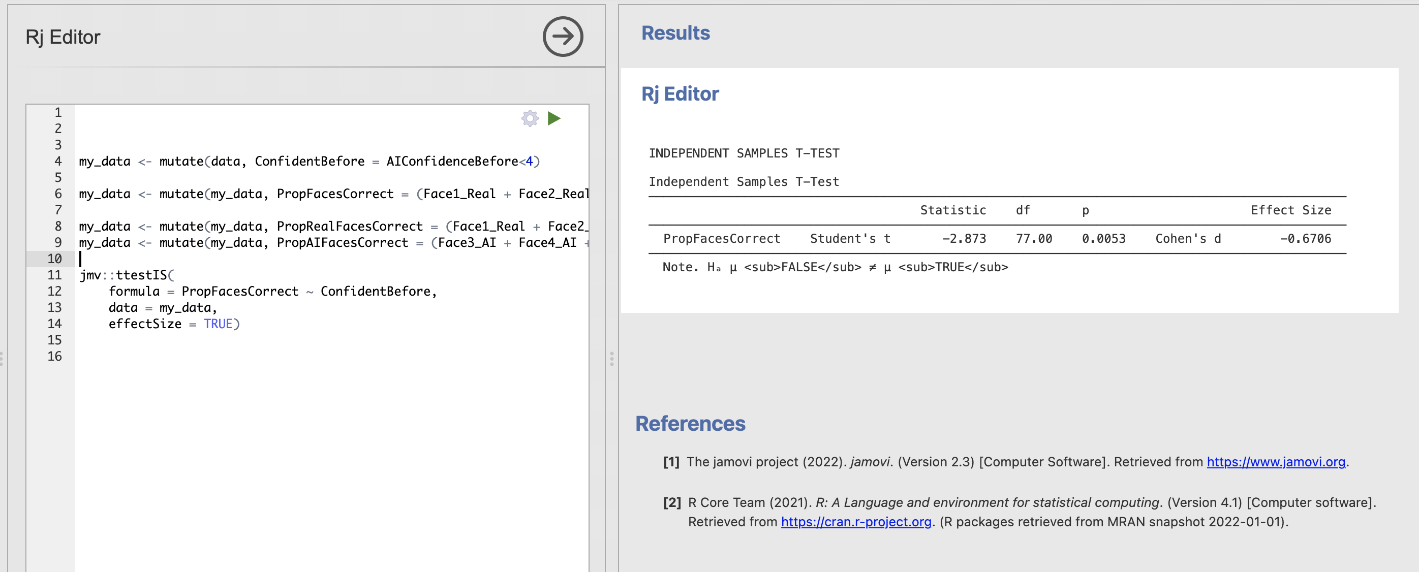
Read through the ttestIS documentation page. How could you change your code to add the following assumption checks

Test for homogeneity of variance
Test for normal distribution

Fill in the blanks to report the results of these tests. Report your results to 3 decimal places.

Shaprio-Wilk’s test for Normality found difference to a normal distribution, W = , p = .

Levene’s test for homogeneity of variance difference in the variances of the two groups, F(,) = , p = .

Based on these results we should report .

The documentation page contains a list of all the possible information that we can pass as an input to our ttestIS() function call. Each item in the list corresponds to the options available in the Jamovi dialogue box.

Have a look at the norm and eqv definitions. What would you need to add to the function call to run these additional checks?

The following code will compute all the checks in addition to the t-test.

jmv::ttestIS(
    formula = PropFacesCorrect ~ ConfidentBefore,
    data = my_data,
    effectSize = TRUE,
    norm = TRUE,
    eqv = TRUE)

The results should look like this:

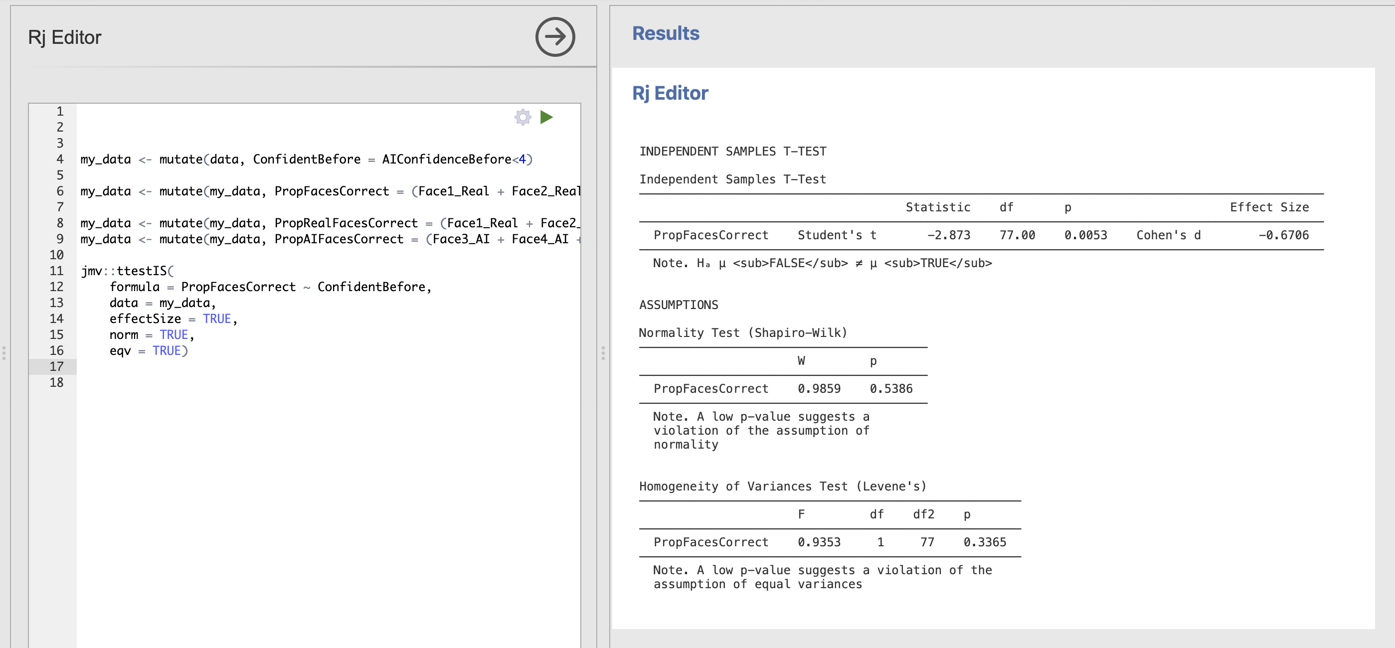
Do the assumptions for Student’s t-test hold for this data?

Your script might be getting quite long at this point! It is always a good idea to keep code neat and tidy where possible so that other people are able to read it, and so that we can read it if we come back to the analysis in the future.

There are many ways to keep things organised in a script. Here are two good hints, code comments can organise your script without changing the output and print() statements can help organise your code and the outputs.

Code comments

Any line of R code that starts with a hashtag is called a ‘comment’. The writing on this line is there for our information and will not be run by the computer. Adding code comments is a useful way to annotate your code indicating what each line or each section is doing. For example:

# This is code comment

# Compute which participants were more confident than the median
my_data <- mutate(data, ConfidentBefore = AIConfidenceBefore<4)

This will make it easier to understand what the coding is doing in future.

Print statements

We can use the print() function to help organise our code as well. The text within the call to print() will not be executed by the computer but will simply be printed into the output console. This can be useful to break the output of your code into sections and to inlcude additional information about the analysis next to the outputs themselves.

For example:

print('Hypothesis 1')
print('Confident people are better at distinguishing AI faces from real faces')
jmv::ttestIS(
    formula = PropFacesCorrect ~ ConfidentBefore,
    data = my_data,
    effectSize = TRUE,
    norm = TRUE,
    eqv = TRUE)

This code will print out information about the hypothesis next to the outputs.

A full cleaned and commented version of our code might look like this.

# Compute which participants were more confident than the median
my_data <- mutate(data, ConfidentBefore = AIConfidenceBefore<4)

# Compute the proportion of all faces each participant got right
my_data <- mutate(my_data, PropFacesCorrect = (Face1_Real + Face2_Real + Face3_AI + Face4_AI + Face5_AI + Face6_AI + Face7_Real + Face8_Real + Face9_Real + Face10_Real + Face11_AI + Face12_AI) / 12)

# Compute the proportion of REAL faces each participant got right
my_data <- mutate(my_data, PropRealFacesCorrect = (Face1_Real + Face2_Real + Face7_Real + Face8_Real + Face9_Real + Face10_Real) / 6)

# Compute the proportion of AI faces each participant got right
my_data <- mutate(my_data, PropAIFacesCorrect = (Face3_AI + Face4_AI + Face5_AI + Face6_AI + Face11_AI + Face12_AI) / 6)

# Hypothesis test
print('Hypothesis 1')
print('Confident people are better at distinguishing AI faces from real faces')
jmv::ttestIS(
    formula = PropFacesCorrect ~ ConfidentBefore,
    data = my_data,
    effectSize = TRUE,
    norm = TRUE,
    eqv = TRUE)

and running this code produces the following outputs including the test from our print statements

Nice and clear what is happening at each stage! There is no perfect or ‘correct’ way to tidy up your code (though some people can get opinionated about this…). Choose a mix of comments and print statements that makes sense to you.

Check Your Understanding

Extend your code to test a second hypothesis.

Confident participants are more accurate than unconfident participants when identifying photos of real faces.

Include some code comments and print statements.

This will require a second indenpendent samples t-test asking whether the mean proportion correct value for only real faces is different between our confident and not-confident groups.

Use the previous t-test as a starting point, can you copy this and modify it to do what we need?

The following code will test the new hypothesis with some comments and print statements

# Hypothesis test
print('Hypothesis 2')
print('Confident participants are more accurate than unconfident participants when identifying photos of real faces.')
jmv::ttestIS(
    formula = PropRealFacesCorrect ~ ConfidentBefore,
    data = my_data,
    effectSize = TRUE)

The output of the whole script should now look like this.

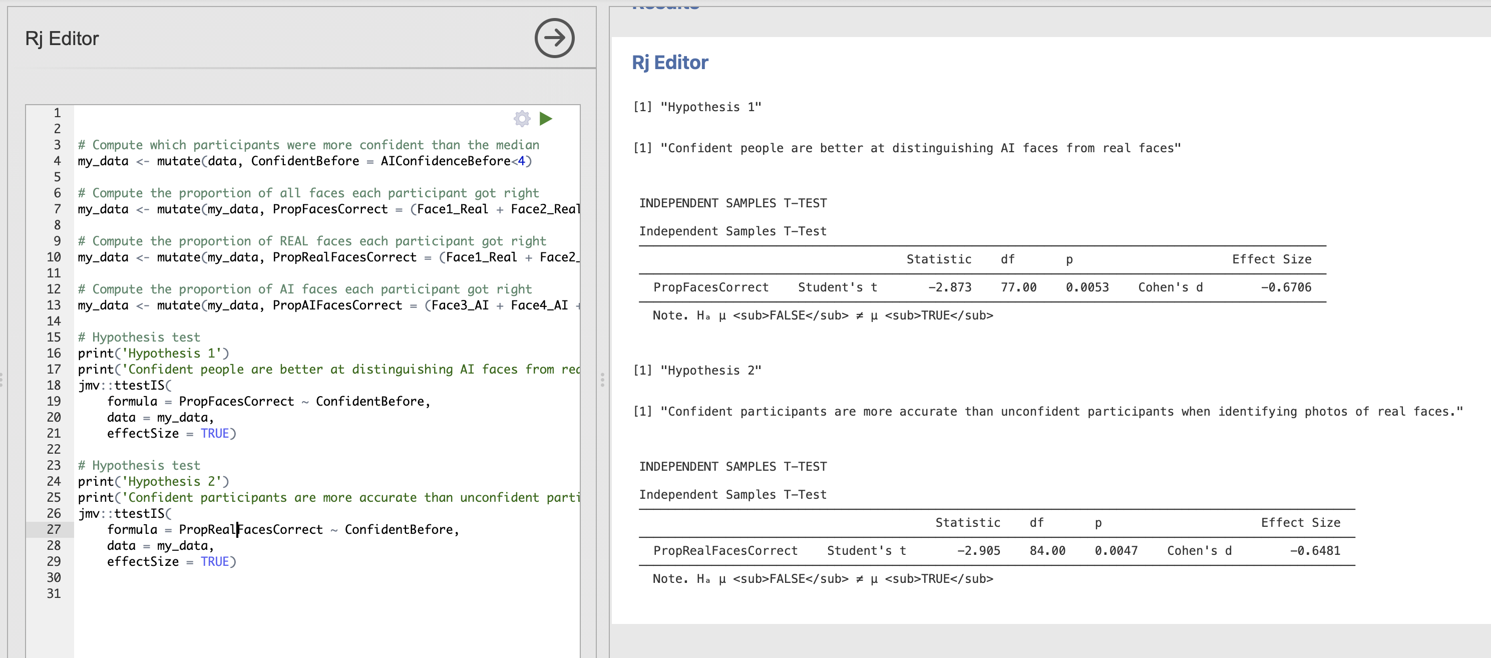
Note how the print statements help to separate the results into interpretable chunks.

5. Analysis from a friend

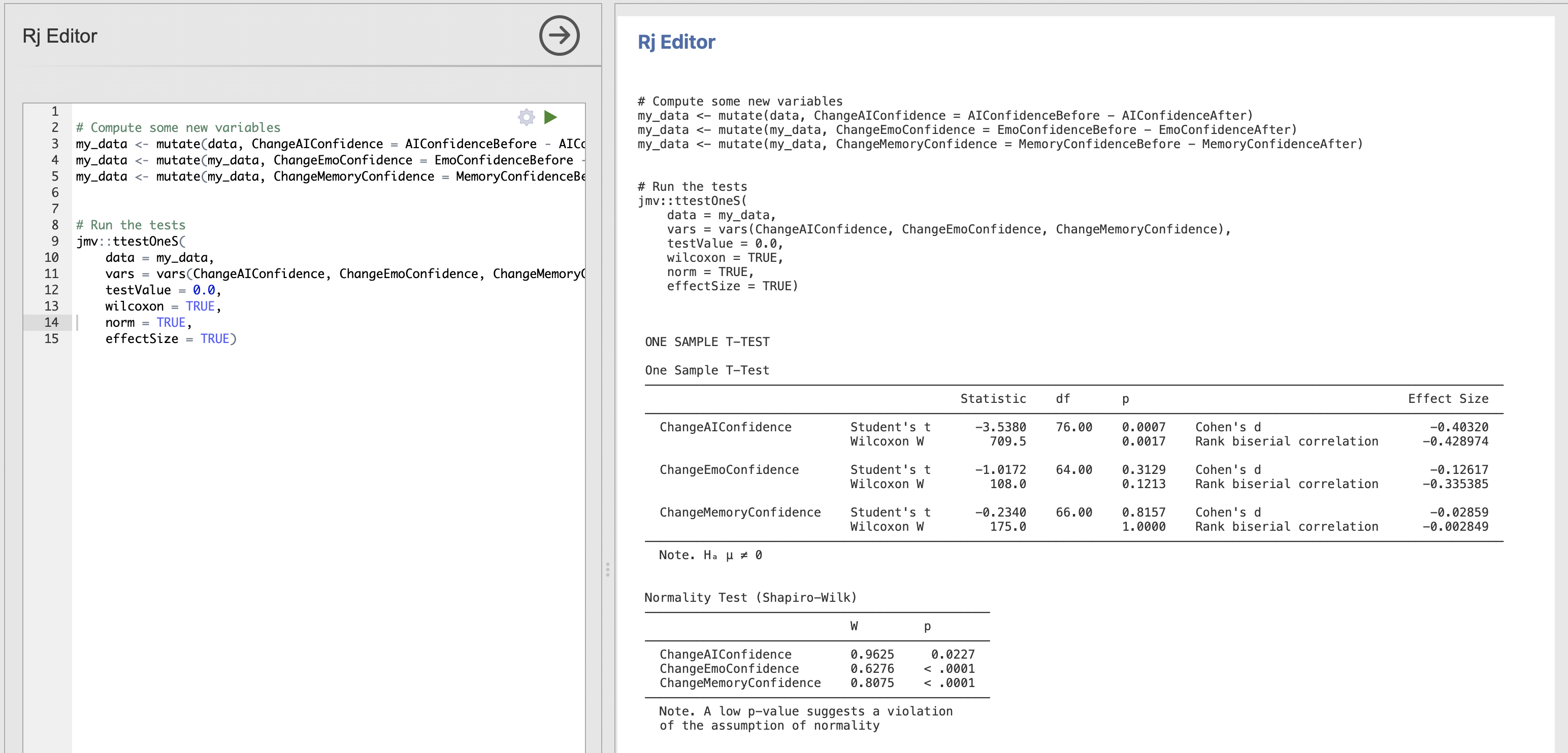
Imagine that of your friends has been running some analyses on this dataset and would like you to check over their work. They send you the following R code that they have put together.

# Compute some new variables
my_data <- mutate(data, ChangeAIConfidence = AIConfidenceBefore - AIConfidenceAfter)
my_data <- mutate(my_data, ChangeEmoConfidence = EmoConfidenceBefore - EmoConfidenceAfter)
my_data <- mutate(my_data, ChangeMemoryConfidence = MemoryConfidenceBefore - MemoryConfidenceAfter)

# Run the tests
jmv::ttestOneS(
    data = my_data,
    vars = vars(ChangeAIConfidence, ChangeEmoConfidence, ChangeMemoryConfidence),
    testValue = 0.0,
    wilcoxon = TRUE,
    desc = TRUE,
    norm = TRUE)

Let’s think about this code a bit, your friend didn’t really explain the plan…

Data Skills - what variables are created?

The code creates three new variables, ChangeAIConfidence, ChangeEmoConfidence and ChangeMemoryConfidence - each is computed by subtracting the confidence values after the face task from the confidence values before the task.

These variables represent the change in confidence from completing the task.

Data Skills - what statistical test is performed?

The code runs a one sample t-test comparing the data mean to 0.0 using the jamovi function jmv::ttestOneS(). The code runs the test on all three variables. We can see that the input vars is passed a list of all three variable names.

Data Skills - what additional computations are performed?

In addition to the t-tests, the code runs a Wilcoxon Rank test, a Shapiro-Wilk test for normality and a descriptive statistics table.

Check Your Understanding

Your friend thinks that none of the confidence values are changed by the task, do you think they are right?

Run the code and fill in the gaps to describe the results.

Variable	Significant or Not	Test Reported
AI Confidence
Emotion Recognition Confidence
School Friend Memory Confidence

Open a new Rj window and run the code above before going any further! Take a moment to read through the code and decide what it is doing.

The results should look like this:

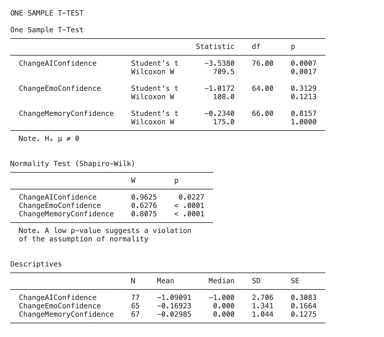
Computing statistics and accurately reporting the results takes a lot of precision! take your time when writing code and results sections - make sure to check and double check your work as you go…

6. Compute effect sizes for t-tests

Let’s think more about effect sizes - computing effect sizes in Jamovi and R is really easy. Simply click the check box to add ‘Effect size’ under the ‘Addtional Statistics’ section of the Jamovi window - or add effectSize = TRUE to the function call in R (we’ve already been doing this above!).

Key step

Update your friend’s code to include computation of effect sizes - the results should appear in the t-test results table on the right.

There are effect sizes computed for every t-test and its non-parametric alternatives.

Cohen’s d is the parametric effect size corresponding to Student’s t-test
Rank Biserial Correlation is the non-parametric effect size corresponding to Wilcoxon’s test.

Though they have methodological differences, these effect sizes can be interpreted in the same way as a measure of the magnitude of an effect.

Remember that this is different to the t-value which is a measure of evidence against the null hypothesis. The important difference is that we can have strong evidence against the null either as the difference is large or if we have measured a small difference very precisely. The effect size only cares about the size of the difference between conditions.

Note that Jamovi/R provide a ‘signed’ effect size indicating the direction of the effect in the same way that a t-statistic does. For the following work we can ignore this sign and focus on the magnitudes only. In other words, we’ll consider an effect size of +0.5 or -0.5 to indicate the same magitude of effect.

The creator of many of our classic effect size measures provided a guideline for what might be considered a ‘small’ or a ‘large’ effect.

Effect Size	Cohen’s d	Interpretation
Small	0.2	Small effect
Medium	0.5	Medium effect
Large	0.8	Large effect

These can be useful guidelines - through they have been criticised strongly for both the arbitrary nature of the thresholds and for over-simplifying interpretation of effect sizes. We can still use them as an informal indicator to help us quickly interpret our results.

Data Skills - Is the effect size for ChangeAIConfidence small, medium or large?

The effect size -0.81 is just below the thresold to be a ‘medium’ effect (ignoring the sign of the effect size). The effect size for the Rank Biserial correlation is similar.

Data Skills - Is the effect size for ChangeEmoConfidence small, medium or large?

The effect size -0.02 is a very ‘small’ effect (we can ignore the sign of the effect size). The effect size for the Rank Biserial correlation is much larger - perhaps as the data is not normally distributed.

Data Skills - Is the effect size for ChangeMemoryConfidence small, medium or large?

The effect size -0.083 is tiny! the Rank Biserial correlation is even smaller…

7. Summary

We have explored some new methods for creating new variables and running t-tests with effect sizes using R code. The R code we wrote is a really clear way to specify how variables were manipulated and which tests were run. Quite complex analyses with several stages can be clearly expressed this way.

Finally, we used effect sizes to explore the power and sensitivity of our experiment and explore the possiblity of a follow up study.

References

Miller, Elizabeth J., Ben A. Steward, Zak Witkower, Clare A. M. Sutherland, Eva G. Krumhuber, and Amy Dawel. 2023. “AI Hyperrealism: Why AI Faces Are Perceived as More Real Than Human Ones.” Psychological Science 34 (12): 1390–1403. https://doi.org/10.1177/09567976231207095.

Week 5 : p-values and effect sizes

1. The Dataset

2. The Challenge

3. Compute new variables with mutate()

Compute the grouping variable

Compute the proportion of correct responses

4. Compute a t-test using R

Code comments

Print statements

5. Analysis from a friend

6. Compute effect sizes for t-tests

7. Summary

References

3. Compute new variables with `mutate()`