Week 1 : Data Handling
This week will serve as a refresher on Jamovi. You will use Jamovi throughout your degree for statistical analysis, so it is very important to refresh your memory on this!
A guide to installing Jamovi on your personal computer can be found here
Learning Objectives
| Quantitative Methods | |
|---|---|
| Recoding scores into groups | |
| Calculating total scores | |
| Calculating means |
| Data Skills | |
|---|---|
| Working with the Jamovi editor | |
| Setting up data files for between- and within-participants designs | |
| Computing descriptive statistics in Jamovi |
Today you will be re-familiarising yourself with the Jamovi interface and its layout / basic functions as well as learning how to set up data for different statistical designs.
Setting up data files and entering data
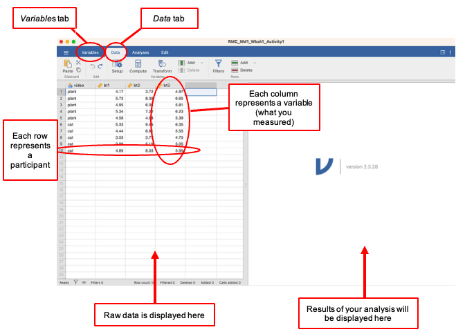
Data are entered into Jamovi using a ‘spreadsheet’ format of rows and columns. When in the Data tab you can view the data. The rows are cases (i.e. participants – each participant gets their own row), the columns are variables (i.e. whatever was measured for each participant gets a column). In the Variable tab rows are the details for each variable (e.g. one row = one variable).
Entering the data in the Data tab is straightforward: you simply type a value in the appropriate box, or ‘cell’.
- The data files for use in the computer practicals are available on the RMC/NM1 Canvas ‘Course Pack’ module. In the text of these pages, the data files will be referred to by file name. You can open different types of data file directly in Jamovi (e.g. .sav or .csv). You can import files directly into Jamovi. There is more information in the Jamovi Textbook
1. Data entry for within- and between-participants or mixed designs
- In a within-participants (or ‘repeated measures’) design the dependent variable (DV) is measured more than once under different conditions or at different times. Therefore, one participant will have two or more scores (e.g. before and after an intervention). This means we need more than one column to record the relevant scores/measurements of the DV.
- For example, in the Data tab: column 1 could be their participant number, column 2 could be their first score and column 3 could be their second score. In the Variables tab you would therefore need three rows to define these variables.
- Participants could provide more than two scores in a repeated measures design.
- In a between-participants design each participant is assigned to a single condition or group. Scores/measurements from two different people can NEVER go in the same row because one row = one person. This means that to identify which condition or group a participant belongs to, we need to assign a label to that participant, which identifies them by their group membership. This is called a grouping variable.
- For example, in the Data tab: column 1 could be the participant number, column 2 could encode which group they were in (e.g. 1 = Experimental Condition OR 2 = Control Group) and column 3 could be their score. In this example, we would need to set up three variables in the Variable tab and for the second row (the group they were in) you would need to define the grouping variable so that you later know what the numbers refer to (e.g. 1 = experimental group, 2 = control group). You could add this information into the description of a variable in the Variables tab.
- Participants could be categorised as belonging to more than on group, e.g. they could be classified according to whether they are studying psychology or neuroscience AND whether they feel confident about using Jamovi or not.
- In some studies, participants belonging to different groups provide more than one score each. Such designs are called mixed designs.
- For example, we might wish to study if a particular intervention helps students feel more confident with their use of Jamovi. This study might record Jamovi-confidence before the intervention and after the intervention. But we might also want to compare the size of the impact of the intervention for students who started off with high confidence to those who started off with low confidence.
Activity 1
Download and open RMC_NM1 Wksh1_Activity1.sav from the Canvas module for the Course Pack
Load the data into Jamovi
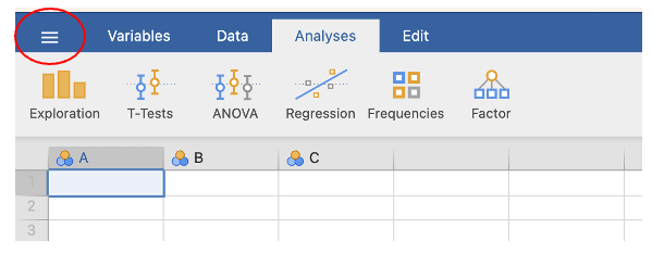
Open Jamovi and click the three horizontal lines in the top left
- Click open - browse
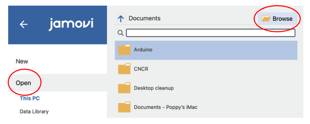
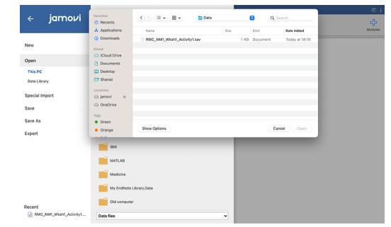
- Navigate to where you saved the data and click to open. Note: when you download the file from the Canvas page it will automatically be saved into your ‘Downloads’ folder so look here if you are struggling to find it.
- Look at the raw data (Data tab) and the variable labels (Variables tab) and answer the following questions.
What is the repeated (within-subjects) variable and how many times is it measured?
The repeated (within-subjects) variable is and is measured times.
Look at the description in the Variables tab
What is the grouping (between-subjects) variable and what are the different groups?
The grouping (between-subjects) variable is and the groups are and .
Look at the description in the Data tab
Understanding the data - visual inspection of the data
Once the data are entered, we need to look at what they can tell us. Jamovi has several tools we can use to better understand the data.
Before doing any statistical analysis, we can look at the data which gives us an idea of what we are dealing with: e.g. How many participants? How many variables? What is the range of scores? Are there any values that seem out of line with the rest?
When satisfied that the raw data look okay, we continue our inspection of the data by using descriptive statistics, such as frequency counts, and measures of central tendency (such as mean, median and mode) and measures of spread (such as range or standard deviation).
Activity 2
Download and open the RMC_NCM_example_output_Explore.sav in Jamovi
Look at the raw data (Data tab) and information about the variables (Variables tab) and answer the following questions.
2. Frequency counts
For nominal and ordinal data, the next step in getting to know the data is to determine the frequency counts for each possible score/value/option, i.e. how often each value occurs (e.g. the number of people who answered “yes” to the question “Did you take Psychology at A-Level?”).
For example, in the dataset RMC_NM1_example_output_Explore.sav, the variable about whether or not a participant took Psychology ‘A’-Level can be examined using this method.
Activity 3a
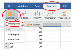
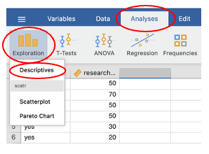
Go to the Analyses menu and choose Exploration
From the submenu, choose Descriptives
- In the descriptives box, choose the variable for which you want to calculate frequency counts and enter it into the box on the right-hand side. Click the tick box next to ‘Frequency tables’ to display the frequency table.
- Answer the following questions based on the Jamovi output
How many valid cases were processed? Was this correct?
cases were processed.
Compare cases to your answer to Activity 2, Q1
Look at the number of times each option occurred. Which was the most common outcome? What percentage of the valid data did this account for?
The most common outcome was and this accounted for % of the data.
3. Crosstabs: looking at frequencies in combinations of groups
Sometimes we want to look at combinations of categories, e.g. how many people studied Psychology at ‘A’-level, how many studied Biology at ‘A’-level, how many studied both, and how many studied neither subject.
For example, in the dataset RMC_NM1_example_output_Crosstabs.sav, the variable about whether or not a participant took Psychology ‘A’-Level and the variable about whether or not a participant took Biology ‘A’-level can be examined using this method.
Activity 3b
Using RMC_NM1_example_output_Crosstabs.sav in Jamovi:
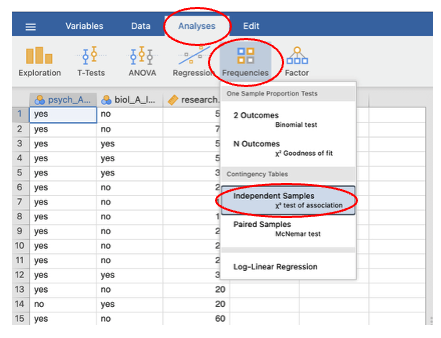
- Go to the Analyses menu and choose Frequencies.
- From the submenu, choose Independent Samples (this is under contingency tables).
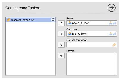
- In the Contingency Tables box, put one categorical variable into the Rows box and the other into the Columns box. (If you have more categorical variables that you want to examine, you add a new Layer for each further variable added).
How many students studied both Psychology and Biology at A-level?
Which was the most common combination of subjects studied?
The most common combination of subjects studied was
4. Exploring the data
Scale data (interval or ratio data) are not always suitable for analysis by frequency counts. Instead, we want to look at measures of central tendency (e.g. means) and measures of spread (e.g. standard deviation). A good way to examine scale data is to ‘explore’ them.
The Exploration module in Jamovi gives a range of statistics including charts to help us see whether the data are normally distributed, whether there are any outliers, and also to get an idea of the spread of the data and their typical value.
While we should always carry out these explorative analyses, we tend not to report them all.
- For example, we do not usually include histograms or stem-and-leaf plots in a results write-up. A good rule of thumb in terms of what we need to report is to think of the exploratory data analyses as being a way in which to check whether our data meet the assumptions underlying successful statistical analysis.
- If they do not meet the assumptions, we need to report how they fail to meet them and state what this means in terms of how we then analyse the data.
The main assumptions which should be met for all parametric tests are:
- The data are at least interval level of measurement.
- The data are normally distributed.
- The variance is homogeneous (similar) between different groups or conditions.
We always have to describe what the data are like in order to carry out a successful statistical analysis. Hence, we routinely report the means and standard deviations of scale data when we carry out statistical tests. (In RMC/NM1, this will be referred to as ‘reporting the descriptives’).
Activity 4
Using RMC_NM1_example_output_Explore.sav in Jamovi:
Go to the Analyses menu and choose the Exploration module.
From the submenu, choose Descriptives.
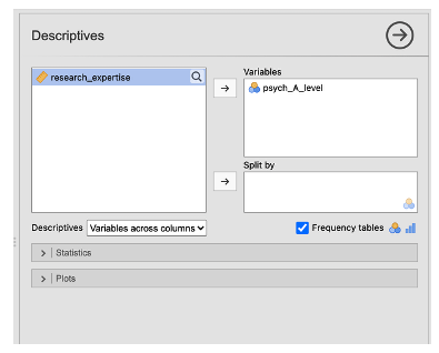
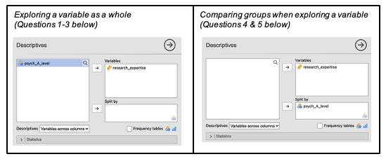
In the Descriptives box, choose the variable(s) you want to explore and enter it (them) into the Variables box on the right-hand side.
- If you want to compare the score on one variable for two or more groups, enter the variable that represents your independent or grouping variable into the Split by box.
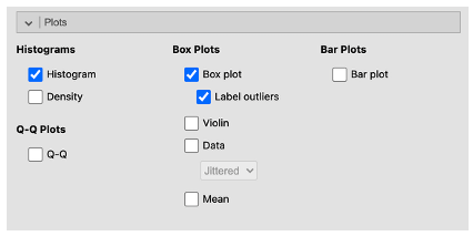
- Click on the Plots menu and select ‘histogram’ and ‘box plot’. Make sure that ‘label outliers’ is selected.
- Answer the questions below based on the results
Are the data normally distributed? (Base your judgement on the histograms.)
The data normally distributed.
Are there any outliers? These will be visible on the boxplots as circles with a number next to them (these numbers indicate which row(s) contains the outlier). Asterisks (*) denote ‘extreme’ values. Write down the row number for any extreme outliers.
If there are any outliers, write the row number for the outlier here
Remove the outlier from the data set by deleting the row with the outlier. Rerun the analysis. Are the data normally distributed?
The data normally distributed.
Rerun the analysis on the data, but this time look at the two groups in comparison (see box above). Does it look as though there are differences between the groups?
Report the means and standard deviations for self-reported expertise for the two groups to 1 decimal place.
Psychology A-level yes: M = , SD =
Psychology A-level no: M = , SD =
Example output
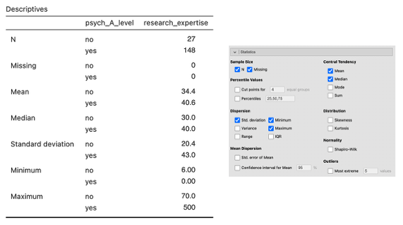
The first part of the descriptives table shows how many cases were processed and if there is anything missing. Look at this to see if the correct number of cases has been processed.
- This can be a useful way to spot if a mistake has been made at the data entry stage and a value has been missed out or added. If the ‘N’ in this table does not match the number of cases expected, double-check the data entry.
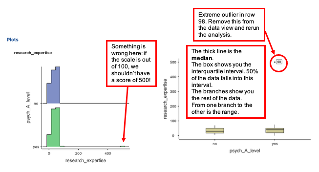
[The output below used ‘research_expertise’ in the Variables box and ‘psych_A_level’ in the Split by box before any extreme outliers were removed.]
- The descriptives table shows number of cases (N), number of missing values (Missing), mean, median, standard deviation, minimum, and maximum. You can change which values you want to display within the statistics drop down menu.
- The output includes two graphical representations. The data from the example look like this as a histogram (left graph) and as a box and whisker plot (right plot). The boxplot gives us less information about the shape of the distribution but provides clear information about the outliers and which scores they are.
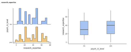
- After you remove the outlier, the histograms and box and whisker plots should look like this:
5. Using Jamovi to prepare/transform data for analysis
When we enter data from questionnaires or have raw data collected from programmes such as Qualtrics or Open Sesame, we often have to prepare the data before analysing it. We might need to:
Calculate total or mean scores for several questions, e.g. for the score on a questionnaire.
Calculate a difference between two scores from the same participant, e.g. when checking if there has been a change from a baseline score.
Combine groups of responses into meaningful categories, e.g. when we want to look at participants with high or low scores on a variable of interest.
We can create these new ‘transformed’ or ‘computed’ variables using Jamovi.
Activity 5
Using RMC_NM1_datagen2.sav in Jamovi
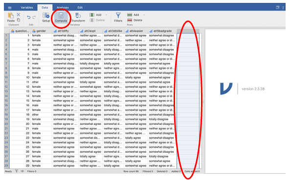
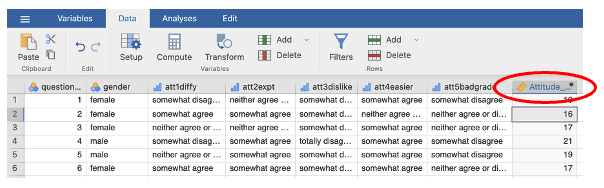
- Click on the column heading of the empty column on the far right of the screen (next to att5badgrade). Go to the Data tab. Choose the Compute option. This will create a new column.
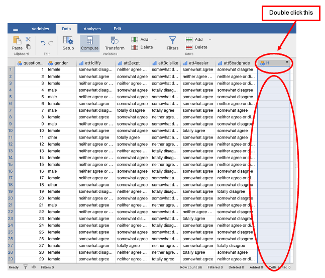
Double click the column heading to open the variable editor.
In the computed variable box, enter a meaningful name for the total score variable (this is the new variable you are calculating).
- Given the nature of the items on this data sheet – look at the labels in Variable View – a name like ‘Attitude_to_Jamovi_total’ would be appropriate to describe the new score.
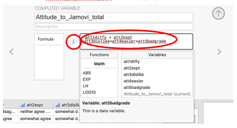
Click the fx box which shows all variables and functions, click the first variable that contributes to your total score to add it to the equation (by double-clicking on the variable name).
Type the ‘+’ sign in the equation box and move the next contributing variable into the function box. Repeat this process, until you have entered all the variables which contribute to the total score.
Back on the data sheet, you should now have a new variable with the computed total score.
- In the Variables tab, describe the new variable appropriately, e.g. enter a descriptive, meaningful label into the description column and check that the level of measurement is correct (scale in this example).
Which participants had the highest score?
Participant ; total score =
Which participants had the lowest total score?
Participant ; total score =
Using the skills from the ‘Understanding the data’ section, decide whether men or women had higher total scores.
had a higher total score (mean females = ; mean males = )
6. Calculate mean scores for several related variables
Activity 6
Using RMC_NM1_datagen2.sav in Jamovi, repeat the process with a new target variable name for the mean score variable.
Go to the Compute module in the Data tab again.
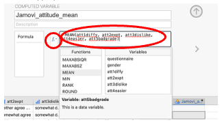
Enter a meaningful name for the mean score variable into the Computed Variable box.
- Given the nature of the items on this data sheet – look at the labels in Variable View – a name like ‘Jamovi_attitude_mean’ would be appropriate to describe the new score.
Click on the fx drop down
In the Functions window, select ‘Mean’ (you will have to scroll down to it). Double click to select it.
Into the Variables window, select the first variable you want in the mean and type a comma next to it. Repeat until all variables are included in the list.
- Back on the data sheet, you should now have a second variable with the computed mean score.
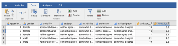
- In the Variable tab define and label the second new variable appropriately.
What is the overall mean (grand mean) for the whole sample (rounded to 1 d.p.)?
The overall mean (grand mean) for the whole sample is (rounded to 1 d.p.)
7. Calculate a difference between 2 scores from the same participant (change from baseline)
Activity 7
Using RMC_NM1_Bloodsugar06-07_for_baseline_calc.sav in Jamovi, calculate a new variable for the change in bloodsugar level from baseline (before) to after a drink has been consumed (after).
- Go to the Variables tab. Choose the Compute option.
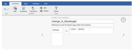
Enter a meaningful name for the difference score variable into the Computed Variable box (this is the new variable you are calculating).
- Here ‘change_in_bloodsugar’ is a meaningful label.
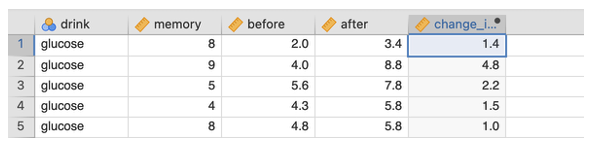
In the fx box double click the ‘after’ variable to move it into the formula box (by double-clicking it). Type the ‘-’ sign on the formula box and move the ‘before’ variable into the formula box. When you calculate the new variable, a positive/greater-than-zero value in the difference variable will mean an increase in the ‘after’ condition compared to ‘before’, and a negative value will mean a decrease.
Back on the data sheet, you should now have a new variable with the computed change in bloodsugar.
- In the Variable View, define and label the new variable appropriately.
Visually inspect the raw data in the change variable. Pay attention to the ‘drink’ variable group. On average does it look as if there is a difference in how bloodsugar changes for the two drink groups?
What did drink group 1 drink? Did their bloodsugar level increase or decrease?
Group 1 drank and their blood sugar
What did drink group 2 drink? Did their bloodsugar level increase or decrease?
Group 2 drank and their blood sugar
8. Recode into different variables to create categories from a continuous variable
Sometimes a continuous variable needs to be recoded to perform a particular analysis, e.g. if you wanted to turn a range of scores from 1 to 9 into three categories, ‘High’, ‘Middle’ and ‘Low’, this is what you need to do on Jamovi.
Activity 8
Using RMC_NM1_datagen3.sav in Jamovi, recode the ‘which_row’ score into a ‘distance_category’ (near, mid, far).
- Go to Data > Transform…
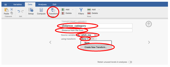
In the drop down next to ‘source variable’, click ‘which_row’. Type a name (e.g. ‘distance_category’) in the ‘transformed variable’ box and describe the variable (e.g. ‘Distance from front’) in the description box.
Click on the drop down next to ‘using transform’ and click ‘Create New Transform…’
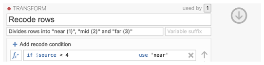
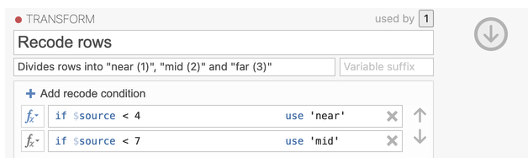
A new window will appear called “Transform”. Give the transformation at name (e.g. ‘Recode rows’).
RECODING lowest values into ‘near’:
Click ‘+ Add recode condition’
This will add a new box at the top which will say ‘if $source … use …’
In this box type the number you want to use as the upper limit for the ‘near’ condition (e.g. if you want to code 1, 2, and 3 as ‘near’, enter ‘< 4’ into the dialog box as this will use all the numbers below, and not including, 4.)
After the word ‘use’, type the value you want to recode the variable to (e.g. Use ‘near’ for the new variable. You need to include the quote marks around the new label.)
RECODING middle values into ‘mid’:
Click ‘+ Add recode condition’
This will add a new box which will say ‘if $source … use …’
In this box type the number you want to use as the upper limit for the ‘mid’ condition (e.g. if you want to code 4, 5 and 6 enter ‘< 7’ into the dialog box as this will use all the numbers below, and not including, 7. Please note that the conditions are executed in order and because we have already set values below 4 to recode to 1, this formula will code values between 4 and 6 as 2. This may take some time to get your head around and this website may help https://blog.jamovi.org/2018/10/23/transforming-variables.html)
After the word ‘use’, type the value you want to recode the variable to (e.g. Use ‘mid’ for the new variable. Don’t forget the quote marks around ‘mid’.)
RECODING highest values into ‘far’:
- The bottom formula box should say ‘else use’. In this box type ‘far’ to recode the remaining values (7. 8, and 9) as ‘far’.
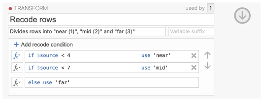
- Back on the data sheet, you should now have a new variable with the recoded data.
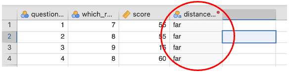
Using the ‘Understanding the Data’ skills, work out how many participants fall into each category
Near:
Mid:
Far:
These calculations of overall scores and recoding techniques will be useful in Research Methods D also