Week 2 : Review of Inferential Tests

Learning Objectives

	Quantitative Methods
	Independent t-tests (and Mann-Whitney)
	Paired samples t-test (and Wilcoxon)
	One-way between participants ANOVA

	Data Skills
	Working with the Jamovi editor
	Setting up data files for between- and within-participants designs
	Computing descriptive statistics in Jamovi

	Open Science
	Working with openly available research data

NoteToday’s session

Below is summary of several of the inferential tests covered at Level 1. As part of your preparation for Level 2 and your Level 3 Project, make sure that you are confident in how (and in what context) to carry out these tests on Jamovi and how to interpret the outputs. Some of the language used here may be a little different from what you learned in RMB but the statistical and theoretical content is effectively the same.

Comparing 2 independent groups on Jamovi

1. Independent t-tests on Jamovi

• An independent t-test is used to assess whether there are significant differences between two independent or separate groups (between-participants design) for a specific measure or DV, e.g. a comparison of psychology and human neuroscience students’ self-rating of statistics expertise.

• In this example, we test the two-sided hypothesis that there is a difference in the self-rated level of research methods expertise of psychology and human neuroscience students in response to a question asking participants to rate their expertise on a scale of 0 to 100.

Walk-through example 1 Using RMC_NM1_WT1_ind_t_test.sav in Jamovi:

1. Screen the data using Exploration.
   1. If it looks as if the whole dataset is normally distributed, proceed with the t-test.
   2. If non-normal, check if this might be due to one or two outliers.
      • If so, remove the outlier(s) and explore the data again. Is it normally distributed now?
      • If not move to Mann-Whitney.

[For the rest of the walk through, follow the instructions for the t-test.]

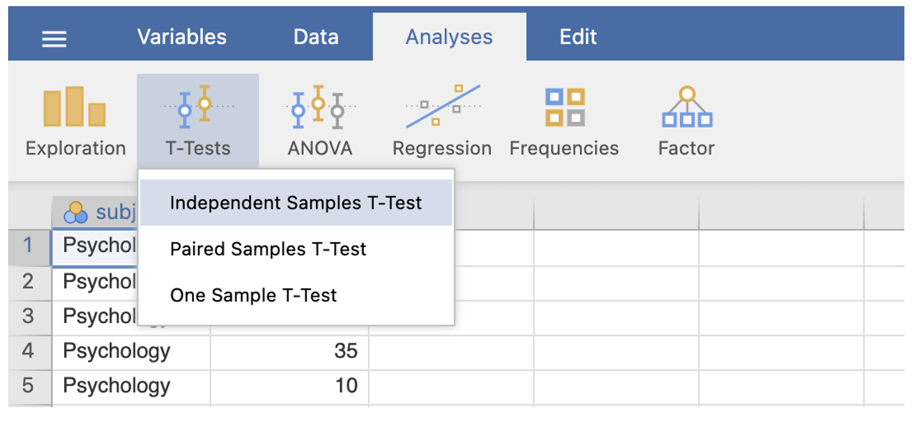
2. Go to the Analyses menu. Select T-Tests. Select Independent-Samples T Test…

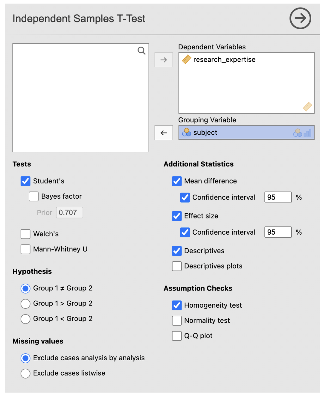
3. In the dialog box, move the dependent variable into the box labelled ‘Dependent Variables’

4. Move the grouping variable into the box labelled Grouping Variable

5. Ensure that ‘Student’s’ is checked

6. Under the additional satatistics menu make sure that the ‘mean difference’ with ‘confidence interval’; ‘effect size’, with ‘confidence interval’; and ‘descriptives’ are checked.

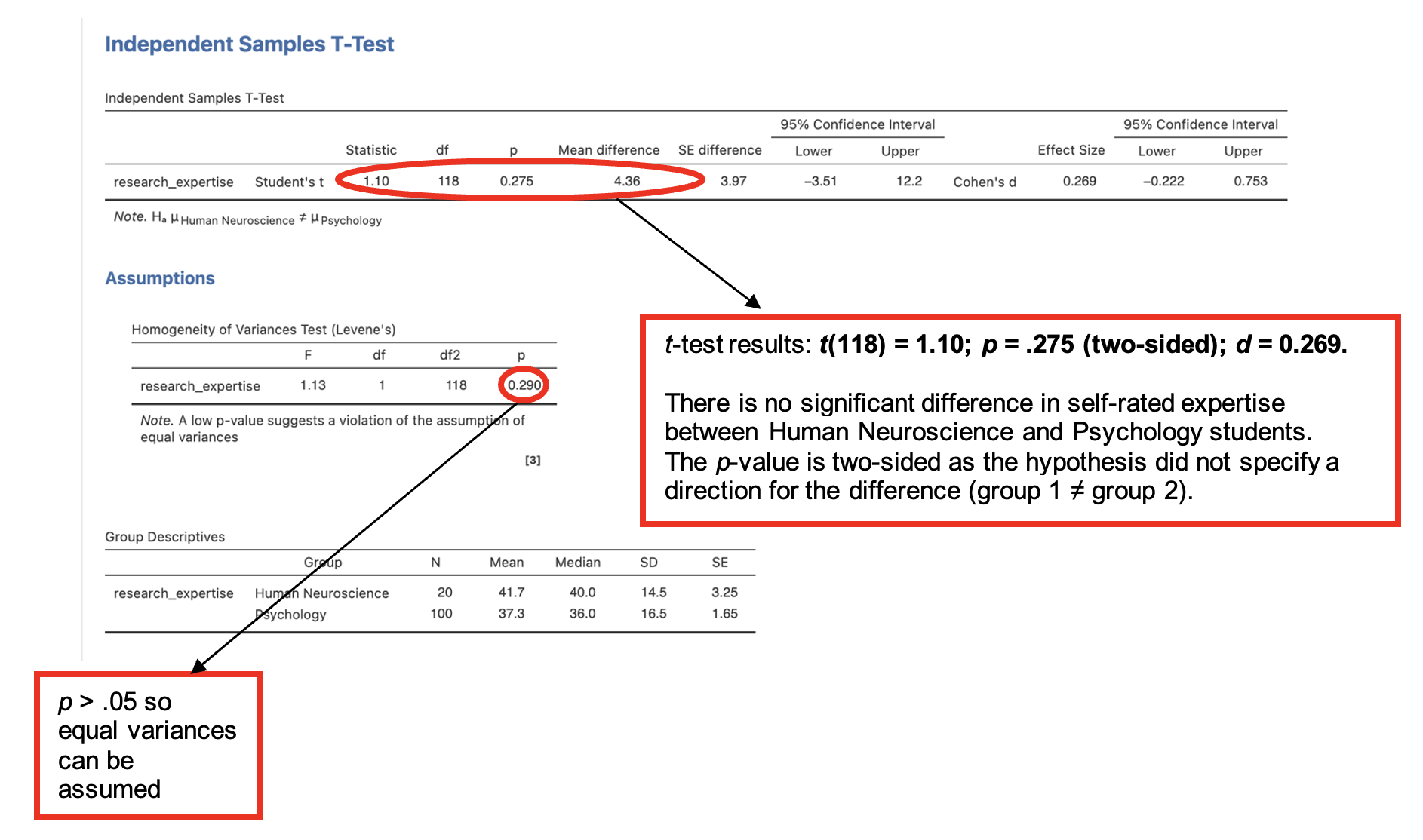
If you have carried out the analysis correctly, your output should consist of three tables. * The Independent Samples T-Test table shows us the results of the t-test. Looking at the first three columns we can determine if the results of the t-test are significant. The next four columns give us some more information about the differences between the two groups. The last four columns provide information about how large an observed effect is. When we report a t-test with a significant outcome, we should also report the effect size. (If the t-test is not significant, you do not need to report Cohen’s d.) - The larger the observed effect, the greater Cohen’s d becomes. Read the value from the Effect Size column. - A common interpretation of effect sizes using Cohen’s d is that d = 0.2 is a small effect, d = 0.5 is a medium effect, and d = 0.8 is a large effect. Essentially, d is measured in units of standard deviations. A d greater than 1 means that the difference between groups is greater than one standard deviation.

• The Assumptions table shows the Levene’s Test for Equality of Variances. This test shows whether the variances of the two groups are equal. When looking at this test, we are testing the assumption that the variances are statistically different. In Levene’s Test…
  • If p is > (greater than) 0.05, equal variances are assumed, and we use the t-test results from the Student’s t-test
  • If p is < (smaller than) 0.05, unequal variances are assumed, and we need to rerun the analysis by clicking ‘Welch’s’ in the Tests menu and use the new values.
• The Group Descriptives table shows the number of participants, the mean score, the median score, and the standard deviations of what we have measured as well as the standard error of the mean for each group/condition. Check here that the groups/conditions match those you intended to compare…

Reporting p-values in RMC/NCM1 * Please give exact probabilities (p=…) to 3 decimal places, wherever possible. You may see very small p-values reported as < .001 but never 0. - This is important as we can never have a p-value of 0. It would mean that there is no chance that the data have come out the way they did by sampling error, which cannot be the case: sampling error is always a possibility.

2. Mann-Whitney (non-parametric) on Jamovi

• The Mann-Whitney test is used when there are different participants in each condition and parametric assumptions are not met. Therefore, it is a non-parametric equivalent of an independent t-test. For example, it can be used with data that are not normally distributed and with data that are ordinal.

• Instead of using means and standard deviations, the Mann-Whitney test looks at the ranking positions of the values from each of the two conditions. The test works out the ranks for the scores in each condition and compares them. The test statistic for a Mann-Whitney test is the U-value.

• In this example, we test the hypothesis that ‘politically correct’ language (pc) makes the ideas expressed feel less familiar to participants compared to ‘non-politically correct’ language (npc). Participants were given as series of sentences and asked to rate them for familiarity of the idea expressed on a 5-point scale (with 1 = very unfamiliar and 5 = very familiar).

Walk-through Example 2 Using RMC_NM1_WT2_Mann-Whitney.sav in Jamovi: a) Screen the data using Exploration. Here the data are not normally distributed (and they are ordinal), so Mann-Whitney is a more appropriate test to use. Record medians for the different groups and minimum and maximum scores. These are needed when reporting Mann-Whitney test results. b) Go to the Analyses -> T-Tests -> Independent T-Test

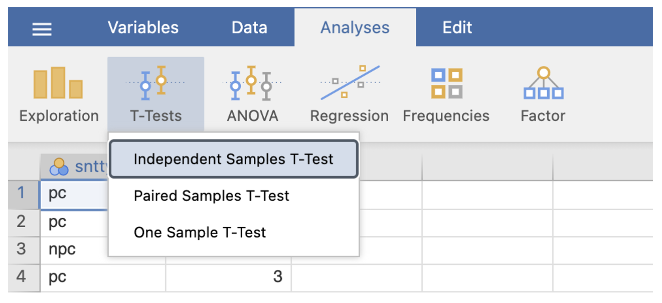
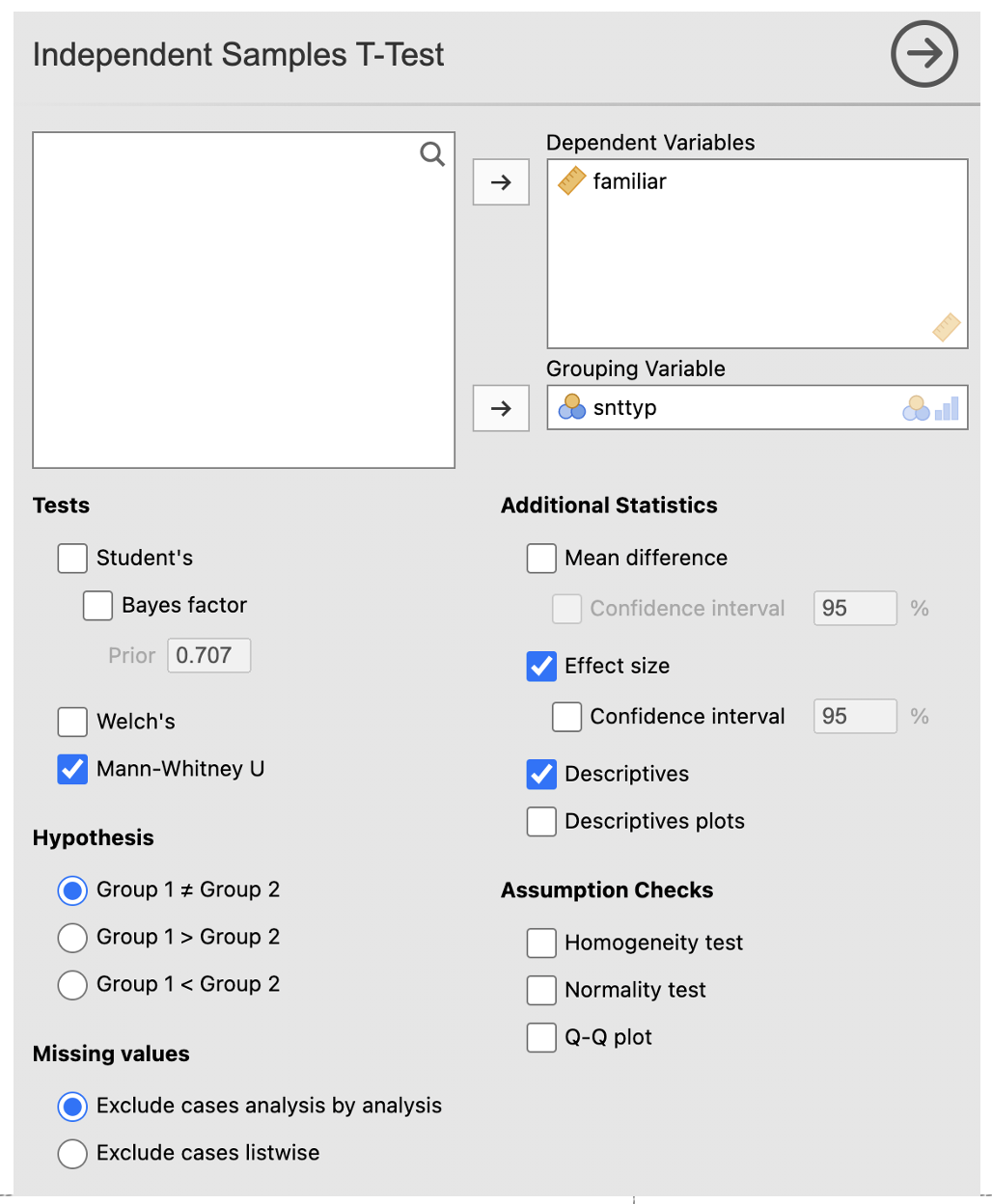
3. Enter the DV into the ‘Dependent Variables’ box. Enter the IV into the ‘Grouping Variable’ box.
4. In the ‘Tests’ section, deselect ‘Student’s’ and select ‘Mann-Whitney U’.
5. Check the box next to ‘Descriptives’ and ‘Effect Size’.

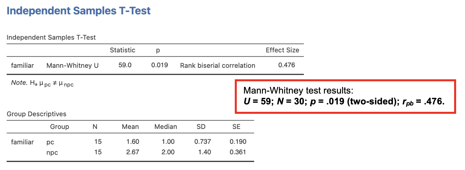
The Jamovi output should look like this: * The Independent Samples T-Test table shows the value of Mann-Whitney’s U to be 59.0. The rank biserial correlation provides a measure of effect size (rpb = .476). The p-value is .019. We conclude that there is a significant difference in familiarity ratings for pc compared to npc sentences. To check the direction of the difference and get some idea of this effect, we would examine the medians for these data. * The Group Descriptives table shows the number of participants in each group and presents the mean, median, standard deviation and standard error of the mean for each group. The mean scores for the groups are NOT reported. Report median scores instead.

Comparing 2 related groups on Jamovi

3. Paired samples t-tests on Jamovi

• A paired samples t-test is used to assess whether there are significant differences between two conditions which were completed by the same, single group of participants (within-participants design or repeated measures), e.g. comparison of a pre- and post-intervention measurement.

• In this example, the hypothesis tested is that people’s performance increased significantly for RMB compared to their performance for RMA (assessed as separate modules). This is a one-sided hypothesis as a specific direction for the difference is predicted.

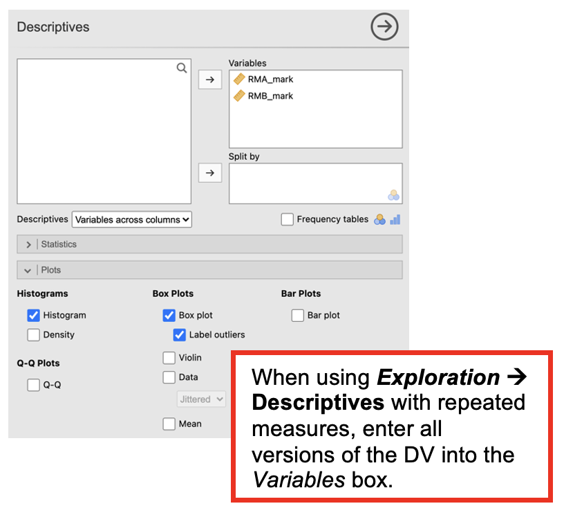
Walk-Through Example 3 Using RMC_NM1_WT3_paired_t_test.sav in Jamovi: a) Screen the data using Exploration -> Descriptives. If it looks to be normally distributed, proceed with t-test. (If not move to Wilcoxon.)

[For the rest of the walk through, follow the instructions for the t-test.]

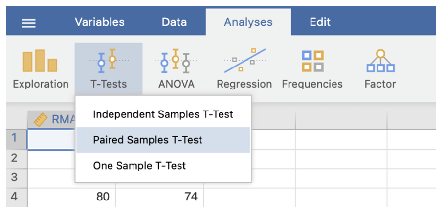
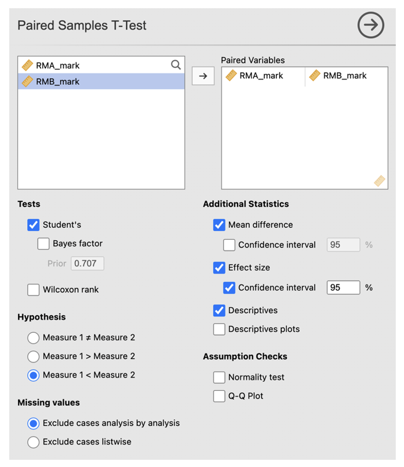
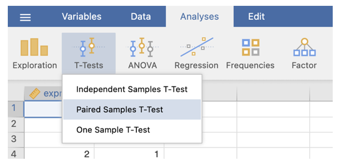
2. Go to the Analyses tab. Select T-Tests. Select Paired Samples T Test

3. Move the first variable of the pair you wish to compare into the Paired Variables box.
4. Repeat with the second variable.
5. Make sure ‘Student’s’, ‘Mean Difference’, ‘Effect size’ and ‘Confidence interval’, and ‘Descriptives’ are checked.
6. As the hypothesis is one-tailed we need to specify this in the Hypothesis section. As we think that scores for RMA will be lower than RMB we should check ‘Measure 1 < Measure 2’ here.

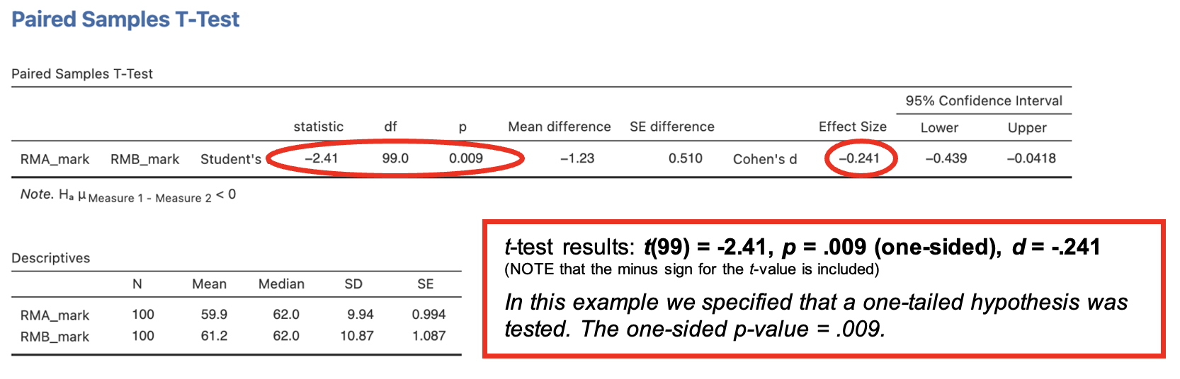
The output of a paired samples t-test consists of two tables. * The Paired Samples T-Test table shows the t-value, the degrees of freedom (df), the p-value, the mean difference between conditions (condition entered first minus condition entered second), the standard error of the difference and effect size information. - When interpreting a one-sided t-test, consider the direction of the difference: is it in the predicted direction? We hypothesised that the RMB mark would be higher than the RMA mark. The direction of the difference suggests that this is the case: The mean difference (RMA mark minus RMB mark) was negative – i.e. RMB mark was higher on average than RMA mark.

• The Descriptives table provides the descriptive statistics for the two conditions: number of participants, means, medians, standard deviations, and standard error of the mean for each condition.

4. Wilcoxon test (non-parametric) on Jamovi

• The Wilcoxon Matched Pairs Signed Ranks Test is used when a paired-samples t-test cannot be used, because the data do not meet the requirements of parametric tests.

• The Wilcoxon test makes use of the fact that the same participants are performing in both conditions. It does this by taking note of the differences in scores for each data-pair. The differences are ranked from lowest to highest.

• Some differences will be positive, some negative, and some 0 (ties) – the latter are ignored as they provide no information. If there is no significant difference between the two conditions, there would be a similar number of positive and negative differences, as the differences between one participant and another would cancel each other out.

• In this example, we test the hypothesis that primary school children recognise more emotions than they express (i.e. spontaneously label or mention) in a story description task.

Walk-Through Example 4 Using RMC_WT4_Wilcoxon.sav in Jamovi:

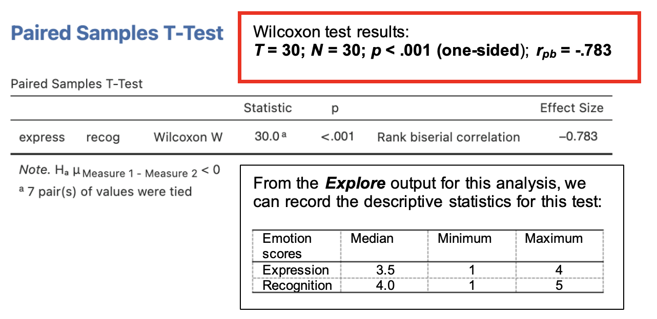
1. Screen the data using Exploration -> Descriptives. Record medians for the different conditions and minimum and maximum scores.
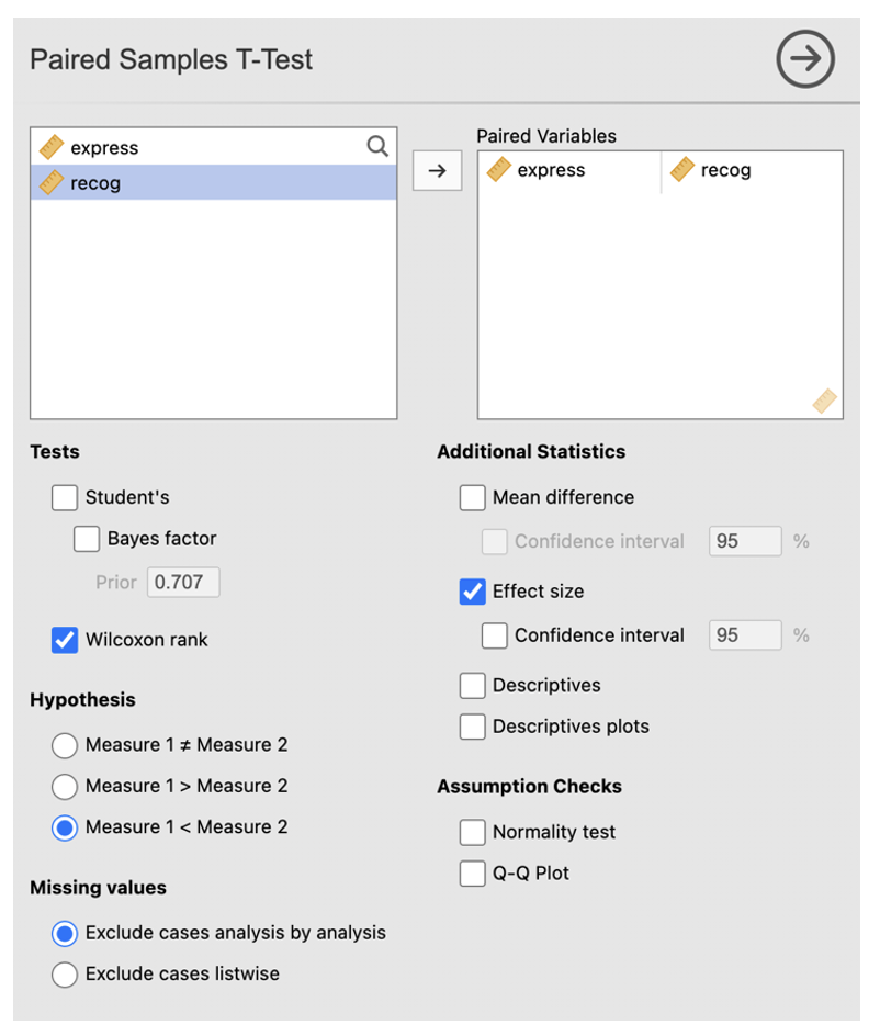
2. Go to the Analyses -> T-Tests -> Paired Samples -Test
3. Enter the first level of the DV into the ‘Paired Variables’ box. Enter the second level of the DV into the ‘Paired Variables’ list.
4. In the ‘Tests’ section, select ‘Wilcoxon rank’.
5. Select ‘Effect size’
6. We have specified a one-way hypothesis that children will recognise more emotions that they express so we should check ‘Measure 1 < Measure 2’.

The Jamovi output should look like this:

• The Paired Samples T-Test table shows the significance of the test. The T-score is under the heading ‘Statistic’. The rank biserial correlation provides a measure of effect size (rpb = -.783). The difference is significant, at p < .001. We conclude that there is a significant difference between emotions expressed and emotions recognised with children recognising more emotions than they express.

TipActivity 1 - Choosing and running the appropriate test

Check Your Understanding - Activity 1 Question 1

Using RMC_NM1_Wksh2_choosing_tests.sav in Jamovi and what has just been covered, test the following hypothesis:

Older students look forward to the module more than younger ones

Test used: independent t-testpaired samples t-testMann-Whitney testWilcoxon test

Is this hypothesis one-sided or two-sided? (Which direction if one-sided?): two-sidedone-sided, group 1 < group 2one-sided, group 1 > group 2

Key descriptives Older students: mean = , median = , sd =

Younger students: mean = , median = , sd =

Report the result If you chose to use a parametric test, fill out the parametric question and if you chose to use a non-parametric test then fill out the non-parametric version

Parametric: t() = ; p = (two-sidedone-sided); d = Non-parametric: U = ; N = ; p = (two-sidedone-sided); r_rb =

Hypothesis accepted? yesno

Check Your Understanding - Activity 1 Question 2

Using RMC_NM1_Wksh2_choosing_tests.sav in Jamovi and what has just been covered, test the following hypothesis:

Psychology students come from large families than Human Neuroscience students.

Test used: independent t-testpaired samples t-testMann-Whitney testWilcoxon test

Is this hypothesis one-sided or two-sided? (Which direction if one-sided?): two-sidedone-sided, group 1 < group 2one-sided, group 1 > group 2

Key descriptives Psychology students: median = , sd =

Human neuroscience students: median = , sd =

Report the result U = ; N = ; p = (two-sidedone-sided); r_rb =

Hypothesis accepted? yesno

Check Your Understanding - Activity 1 Question 3

Using RMC_NM1_Wksh2_choosing_tests.sav in Jamovi and what has just been covered, test the following hypothesis:

Performance scores are higher after practice than before practice.

Test used: independent t-testpaired samples t-testMann-Whitney testWilcoxon test

Is this hypothesis one-sided or two-sided? (Which direction if one-sided?): two-sidedone-sided, measure 1 < measure 2one-sided, measure 1 > measure 2

Key descriptives Before practice: median = , sd =

After practice: median = , sd =

Report the result T = ; N = ; p (two-sidedone-sided); rrb =

Hypothesis accepted? yesno

Comparing more than 2 groups on Jamovi

• This section is about reviewing how to carry out one-way ANOVAs (for data that meet parametric assumptions) in Jamovi.

• One-way ANOVAs have a single factor (IV) which has more than two levels (groups), and a single DV.

• One-way ANOVAs are carried out differently in Jamovi depending on whether the IV is a within- or between-participants factor. You will have had some experience in RMB with one-way between-participants ANOVA – i.e. comparing two or more groups. The following sections go over how to perform one-way between-participants ANOVA. In the next workshop, one-way within-participants ANOVA will be introduced.

Between-participants one-way ANOVA (independent samples)

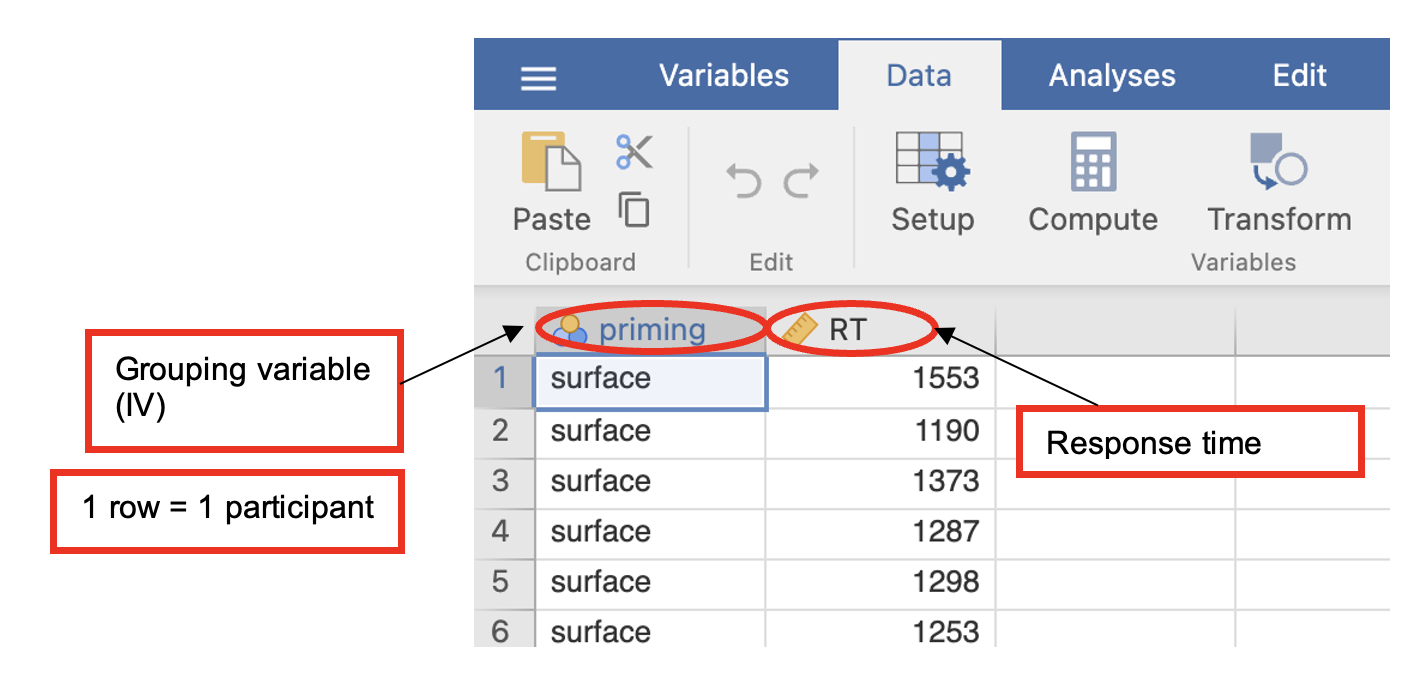
• In this example experiment, students were asked to decide which category a displayed word belonged to (e.g. Is ‘horse’ an animal or furniture?). Response times were recorded.

• Before the categorization task, the participants performed 1 of 3 priming tasks:

  • The “surface” group looked at a list of words and decided if each one contained an ‘e’.
  • The “deep” group looked at a list of words and decided if each one was a living thing.
  • The “no prime” group did not look at any words before (control group).

• Hypotheses tested were:

  • Participants who have previously processed a word at a deep level will categorise it more quickly than those who have processed it at a surface level or in the no prime condition.

  • If surface processing has any effect on later categorization, the response times in the surface condition should be faster than in the no prime condition.

Walk-Through Example 5 “The effect of priming on a categorization task” a) Download and open the RMC_NM1_1way_between_ANOVA.sav from the Canvas folder. b) Click on the “Data” tab and look at the values in the ‘priming’ and ‘RT’ column.

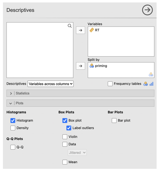
3. Click Analyses -> Exploration -> Descriptives. In the dialog box, enter the DV into the ‘Variables’ box. Enter the IV into the ‘Split by’ box.
4. Go to ‘Plots’. Check ‘Histograms’ and ‘Box plot’ with ‘Label outliers’.

NoteNote

In this example the data are broadly normally distributed with no major outliers and so meet data requirements for ANOVA.

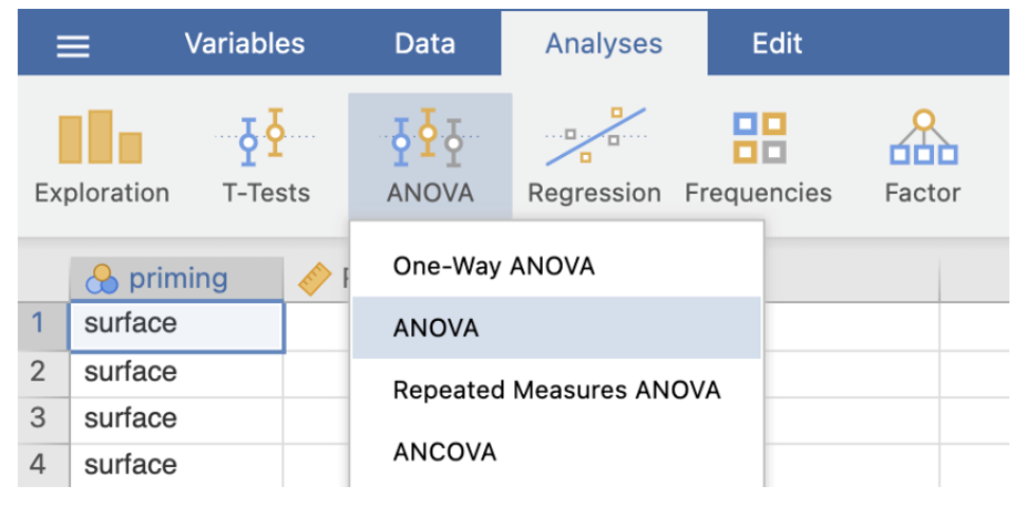
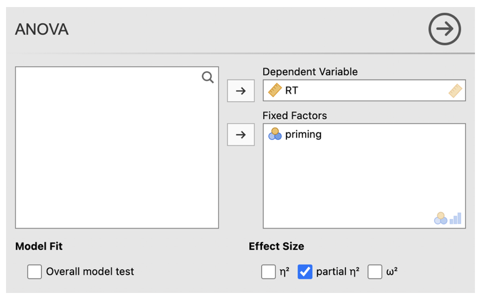
5. Go to Analyses -> ANOVA -> ANOVA

6. In the dialog box, enter the DV into the ‘Dependent Variables’ box. Enter the IV in the ‘Fixed Factors’ box.
7. Under Effect Size check the ‘partial η²’ box.

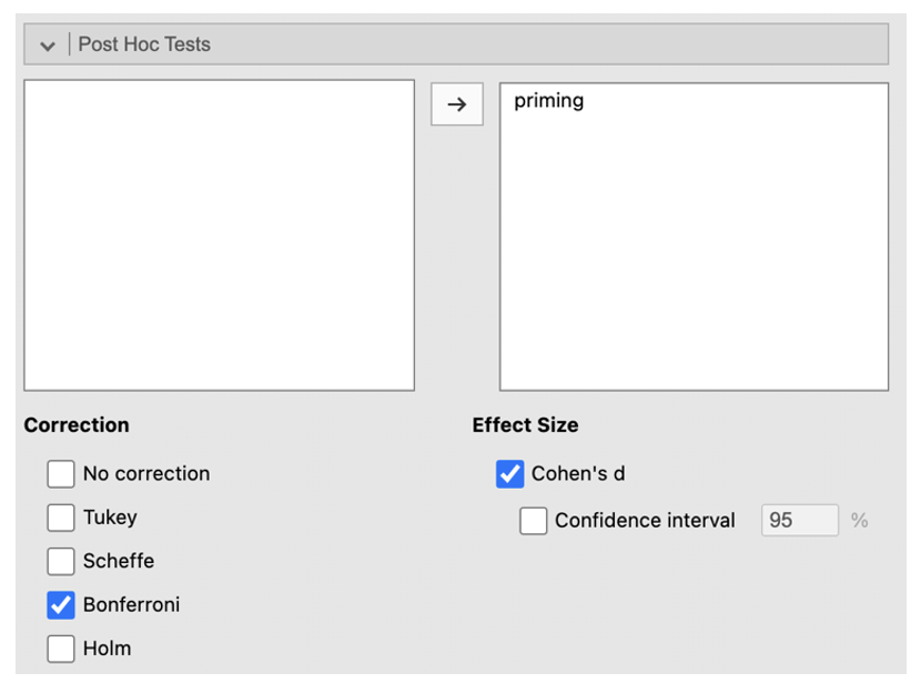
8. Click on the ‘Post Hoc Tests’ menu. Add ‘priming’ to the right-side box. Select ‘Bonferroni’ under ‘Correction’ and check the ‘Cohen’s d’ box under Effect Size.

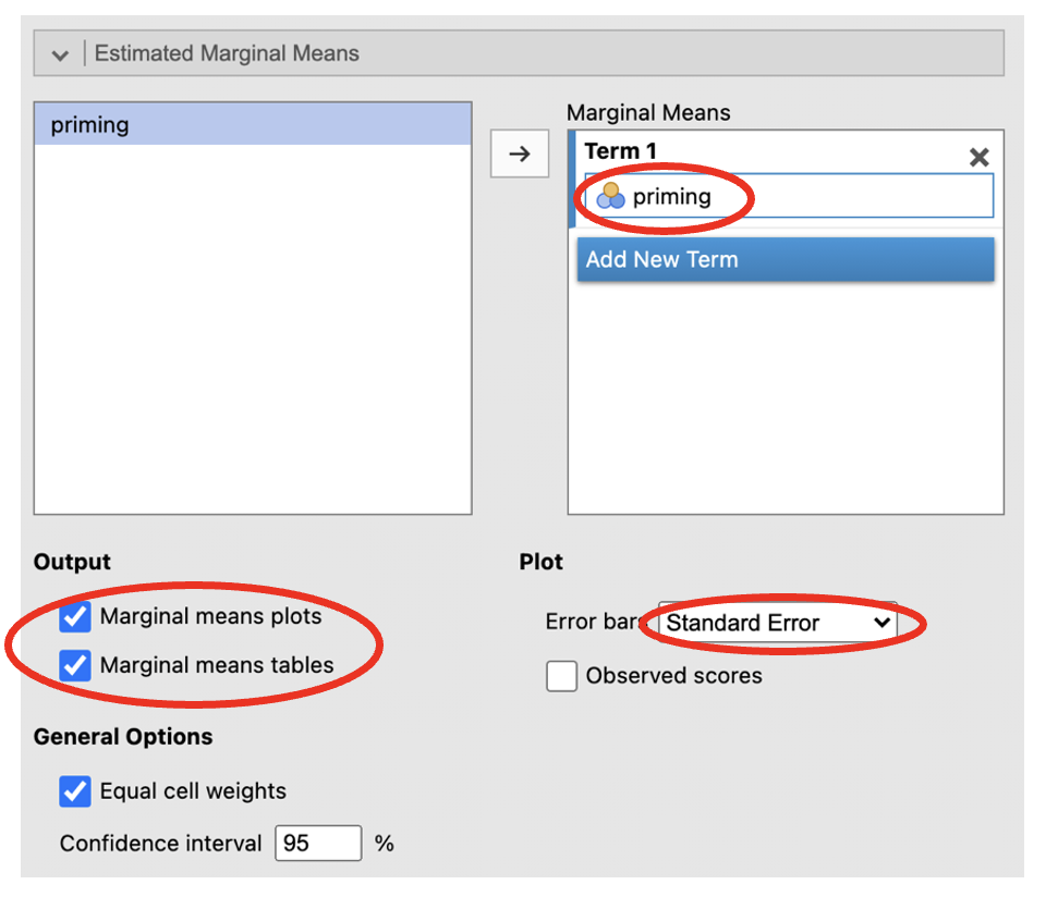
1. Click on the ‘Estimated Marginal Means’ menu. Add ‘priming’ to the ‘Term 1’ box. Select ‘Marginal means plots’ and ‘Marginal means tables’ under ‘Output’ and change the ‘Error bars’ drop down to ‘Standard Error’.

Jamovi output: One-way ANOVA between-participants

• The means and standard errors for each group can be found in this table (scroll down as this will be at the bottom). The standard deviations and number of participants in each group can be found in the descriptive exploration we did earlier.

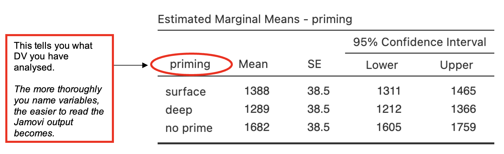
From this table and the Descriptives table from performing the Exploration analysis answer the following questions:

TipJamovi Output One-way ANOVA (between) questions

Question 1

Which priming group responded the fastest? surfacedeepno-prime

Question 2

Which priming group responded the slowest? surfacedeepno-prime

Question 3

Which group showed the largest variation in response time? surfacedeepno-prime

• The ANOVA table shows if the mean differences between the levels/conditions of the IV are statistically significant.

TipJamovi Output One-way ANOVA (between) questions

Question 4

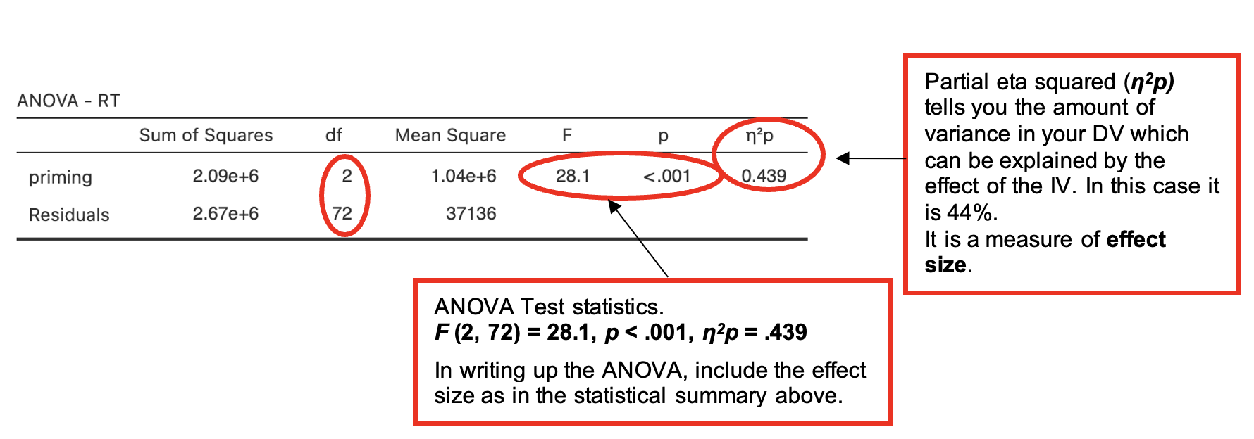
Is there a significant effect of priming upon response times in the categorization task? yesno

• The next table presents the post-hoc test and looks at the mean differences between conditions to determine which of these differences are statistically significant.

TipJamovi Output One-way ANOVA (between) questions

Question 5

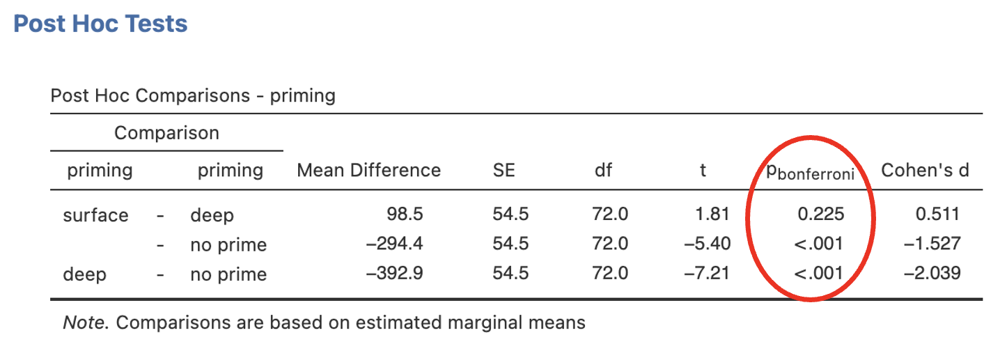
Which (if any) condition(s) is significantly different from “no prime”? surface and deepsurface onlydeep onlyneither are significant

Which (if any) condition(s) is significantly different from “deep”? surface and no primesurface onlyno prime onlyneither are significant

• The final part of the output is a plot of the means which is a useful tool to understand the differences between groups. The white circles represent the mean and error bars represent whatever you have set them to (standard error of the mean in this case).

Figure 1 Mean Categorisation Times (ms) for the Surface, Deep and No-Prime Conditions

NoteNote

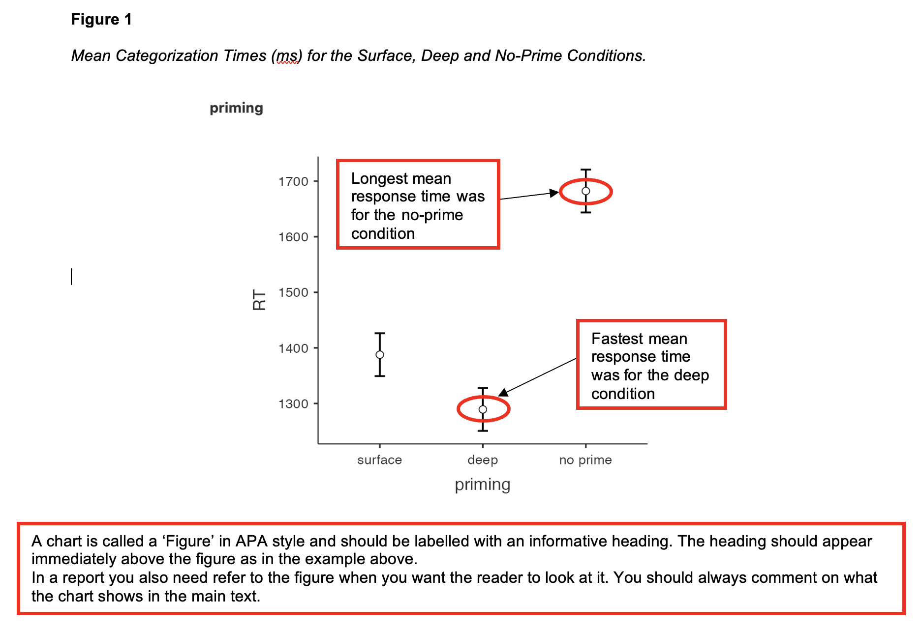
A chart is called a ‘Figure’ in APA style and should be labelled with an informative heading. The heading should appear immediately above the figure as in the example above. In a report you also need refer to the figure when you want the reader to look at it. You should always comment on what the chart shows in the main text.

Writing up the ANOVA

• In reporting ANOVA results, include:
  • Information about the descriptive statistics for the different groups, possibly including a figure to illustrate the findings
  • A summary of the test statistic including probability and effect size
  • Comment on whether the findings supported the hypothesis or not.
• Here is an example write-up for the ANOVA in Walk-Through Example 5. (This report includes a table of means instead of a figure)

TipOne-way ANOVA Write Up

Fill in the blanks

(Any data preparation, e.g. how the response times were calculated or how the data were trimmed or if and how many outliers were removed, should be presented in the section of the method about data preparation and data analysis.)

In a report, an ANOVA results section could look like this:

Results

As predicted, the mean categorization times were lowest in the ‘deep’ group, followed by the ‘surface’ group, with processing times being slowest in the ‘no prime’ group. A one-way between-participants ANOVA found significant differences in categorization times between the three priming conditions (see Table 1).

Table 1 Means (Standard Deviations in Parentheses), and One-Way Analysis of Variance Statistics for Categorization Times (ms) for the Priming Conditions.

Measure		Priming Condition		F(2,[])	η2p
	Surface	Deep	No-prime
Categorisation time	(141)	1289 (223)	1682 ()	28.1***	.44

*** p < .001

To locate these differences, a Bonferroni post hoc test was performed. The surface and no prime groups differed significantly (mean difference = 294 ms, p < .001) as did the and no prime groups (mean difference = 393 ms, p < .001). However, there was no difference between deep and priming (mean difference = 99 ms, p = ).

These findings supportpartially supportdo not support the hypothesis in that both surface and deep priming led to an advantage in the categorization task compared to the no prime condition, but there was no evidence that deep priming produced a greater advantage than surface priming.