Week 8 : Linear Regression

Learning Objectives

1. Decide when it is appropriate, based on the shape of your data, to use linear regression.
2. Use Jamovi to conduct a linear regression, interpret the output and write up the findings in APA format.

NoteExamining your data to decide if using linear regression is appropriate

When conducting a correlation analysis or a linear regression, there are several assumptions which need to be met in order for the analysis to be meaningful.

Checking assumptions for linear regression

For each of the following data sets, run checks to see if the assumptions for linear regression are met. (HINT: You may wish to draw on Jamovi techniques used in the first RMD workshop)

TipTest your understanding

A and B

Run the appropriate tests on the data in variables A and B in LR_assumptions.csv

1. Does the relationship look linear? YesNo

2. Does the data have evenly distributed variances (is it homoscedastic) YesNo

3. Are there any outliers? YesNo

4. Overall is it appropriate to run a linear regression on these data? YesNo

A and C

Run the appropriate tests on the data in variables A and C in LR_assumptions.csv

1. Does the relationship look linear? YesNo

2. Does the data have evenly distributed variances (is it homoscedastic) YesNo

3. Are there any outliers? YesNo

4. Overall is it appropriate to run a linear regression on these data? YesNo

C and D

Run the appropriate tests on the data in variables C and D in LR_assumptions.csv

1. Does the relationship look linear? YesNo

2. Does the data have evenly distributed variances (is it homoscedastic) YesNo

3. Are there any outliers? YesNo

4. Overall is it appropriate to run a linear regression on these data? YesNo

A and E

Run the appropriate tests on the data in variables A and E in LR_assumptions.csv

1. Does the relationship look linear? YesNoYes, but not if you take the outliers into accountNo the outliers are an issue

2. Does the data have evenly distributed variances (is it homoscedastic) YesNo

3. Are there any outliers? YesNo

4. Overall is it appropriate to run a linear regression on these data? YesNo

Using Jamovi to carry out a Linear Regression

Open attract.csv. The idea with this made-up data set is that it tests the assumption that we can predict the number of dates a person has been on from their attractiveness rating on a scale of 1 to 10.

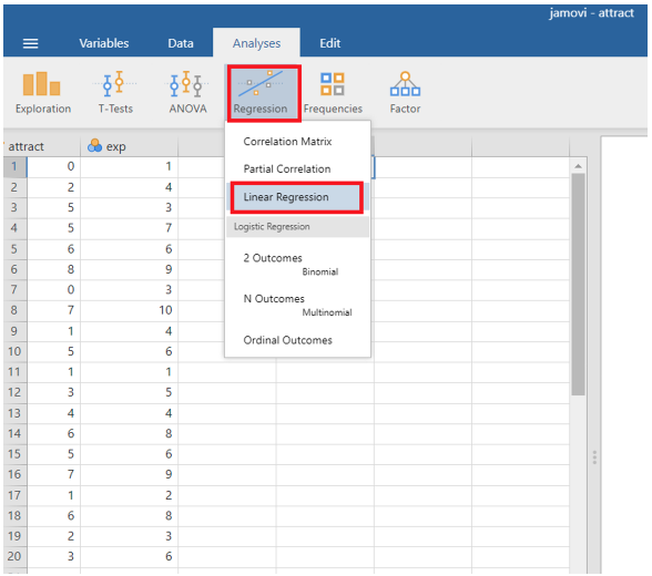
1. In Jamovi, once you have checked that the data are suitable for linear regression, go to Analyses > Regression > Linear Regression

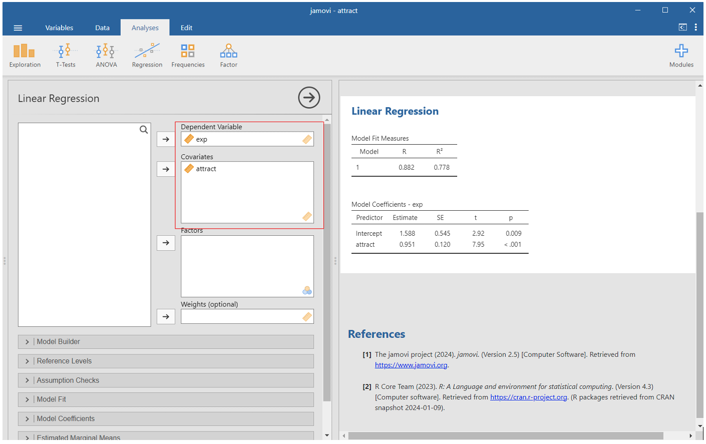
2. In the “Linear Regression” window, move your predictor variable to the Independent(s) panel and the predicted variable to the Dependent panel.

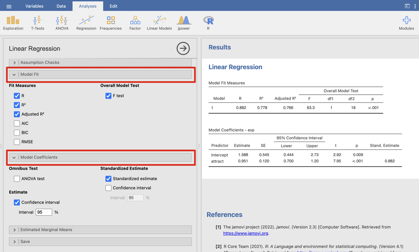
3. In the Linear Regression tab Model fit tick R, R², adjusted R² and F test. Under Model Coefficients click confidence interval and standardised estimate.

4. The result is shown in the right panel. Look at the notes to help you interpret.

Coefficients

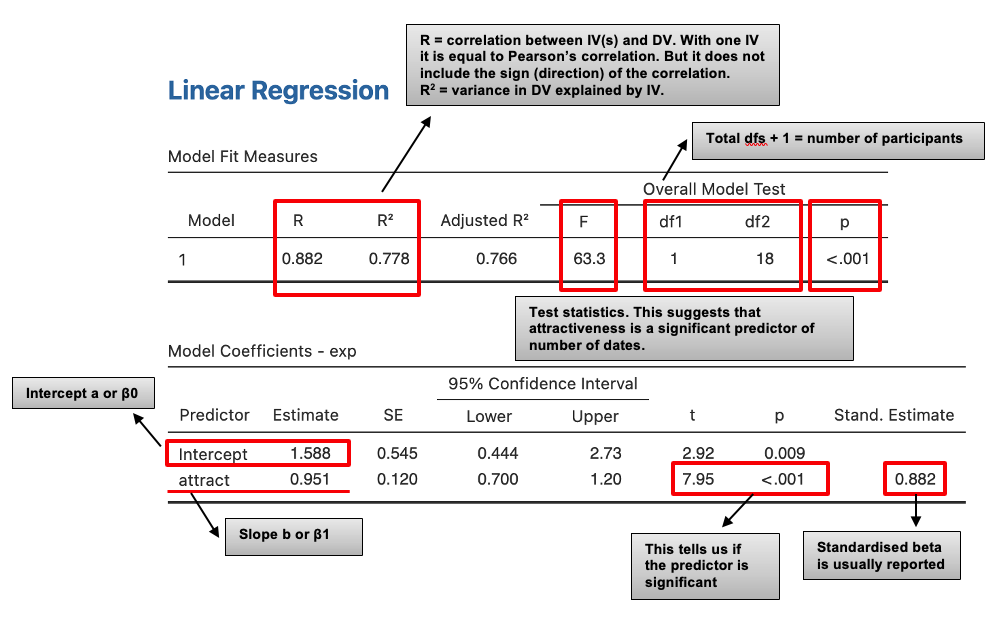
The coefficients table gives us details of the model parameters (beta values, i.e. the slope of the line and the intercept) and the significance of these values.

β0 = 1.588 – a indicates that for someone with an attractiveness rating of 0, the model predicts you will have been on just over 1.5 dates

β1 = 0.951 – this is the slope of the regression line and represents the change in the outcome associated with a unit change in the predictor (positive number means positive regression line, negative number indicates negative regression line).

So if your attractiveness increased by 1, this would predict an increase in number of dates attended by 0.951 (although remember that attractiveness only accounts for 78% of the variance in number of dates, so you may be lucky if you also have a sense of humour!).

The regression line for this analysis therefore has the following equation:

\[ y = 1.588 + 0.951x \]

Adding a line of best fit to a Jamovi scatter plot

Using the attract.csv data, create a scatter plot. In Jamovi click on Exploration > Scatterplot.

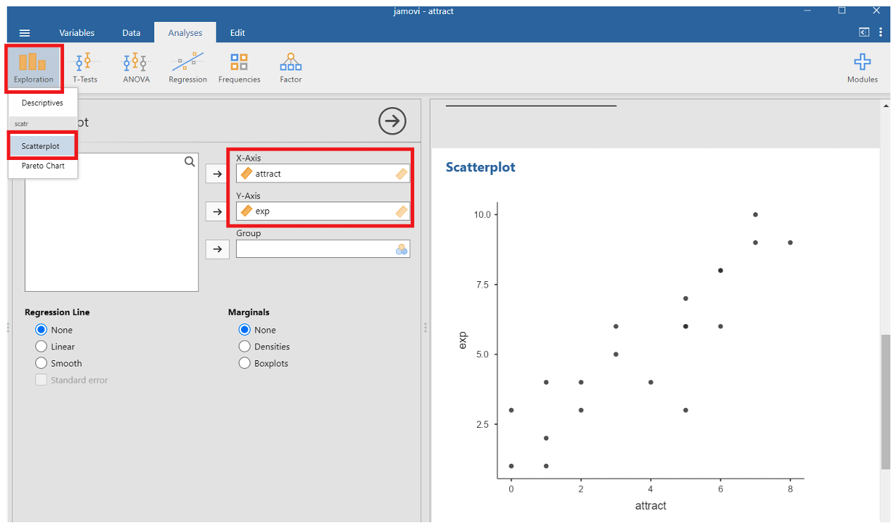
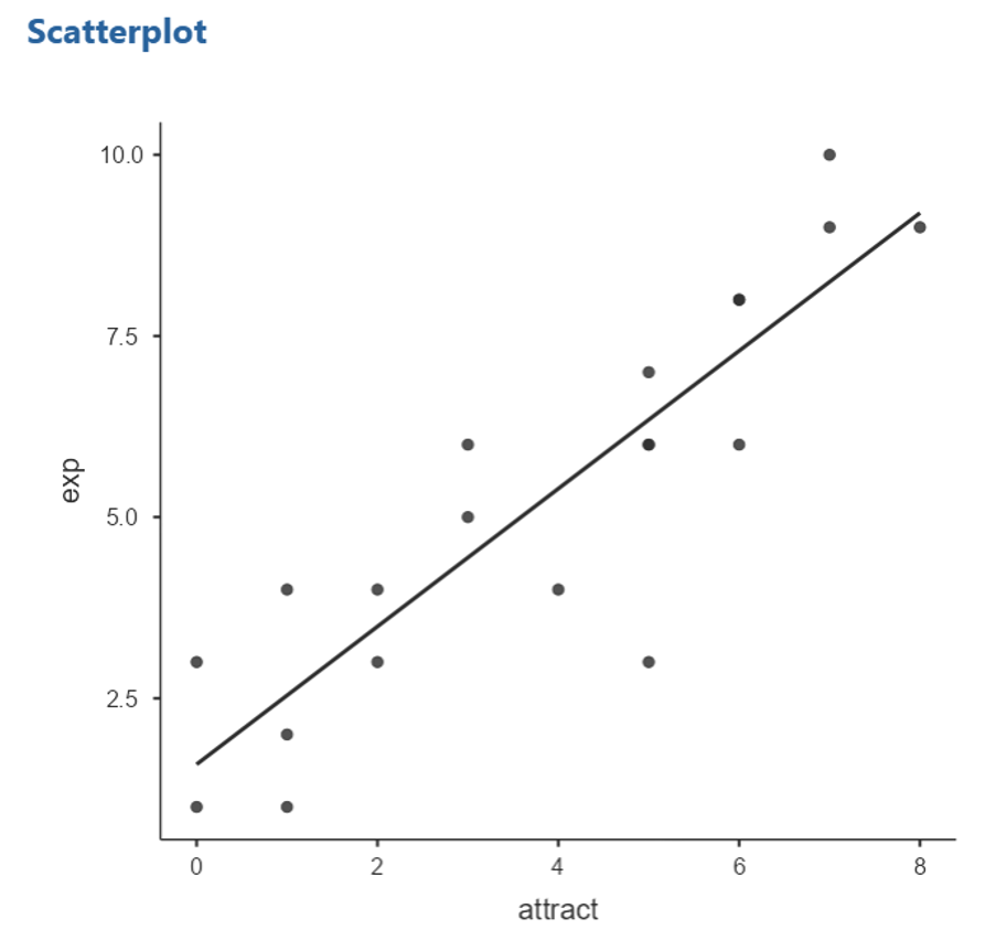
To get the line of best fit, select Linear under the Regression Line options

How good is the prediction?

There are a number of ways to assess the quality of predictions that can be made using the equation produced by a regression analysis.

• R² corresponds to the predictive power of the relationship between predictor and criterion. For a simple linear regression, R is the same as the correlation between the two variables, but it does not give the sign (direction) of the correlation. If R² is high then most of the variance in the actual values of the predicted variable is explained by the prediction and the regression is good.

• ‘R² adjusted’ measures the predictive power of the regression equation for the population rather than the sample (that is for values not in the original data set, but part of the same population).

• The ANOVA in regression. The null hypothesis for this ANOVA is that there is no relationship between the actual values of the predicted variable and the values given by the prediction. If the p-value is less than .05 we can be confident that the relationship between the two variables is a significant one.

Writing up the Linear Regression

“A linear regression was used to examine the relationship between attractiveness and the number of dates someone had been on. The regression equation produced a good fit with the data (R² = .778), indicating that, as hypothesised, someone’s attractiveness score was a good predictor of the number of dates they had been on, F(1, 18) = 63.252, p < .001.

There was a significant positive relationship between attractiveness and number of dates (β = 0.882; t = 7.953, p < .001) with number of dates increasing with increases in level of attractiveness. The model predicts that one unit change in attractiveness would result in an increase in dates attended of 0.951.”

Transferable Skills: Linear Regression

Interpreting Statistical Outputs from Different Software Platforms (e.g. SPSS)

Occasionally, you might need to interpret statistical outputs which have been generated using different statistical software, such as SPSS. Below you will see an example SPSS output which investigated if the researchers could predict levels of worry about statistics using hours of study engagement (e.g. hypothesising that as hours of study engagement increased, worries about statistics would decrease). Look at the output below to see what you can interpret based on what you know about linear regression so far.

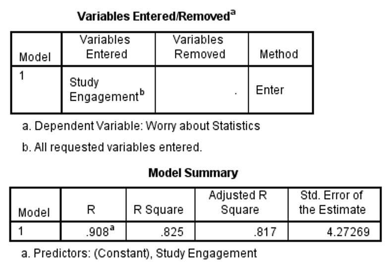
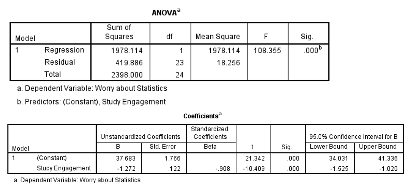
Based on this output, we can tell that 82% of the variance in worries about statistics could be explained by hours of study engagement (e.g. see the adjusted r square value in the model summary box). We can also see that hours of study engagement was a significant predictor of worries about statistics. Note that older versions of SPSS report p < 0.001 as .000. Make sure this doesn’t through off your interpretation, it still means p < .001!

Writing up the Jamovi Output

The file stress.csv contains some made-up data on people’s lifestyles and stress. We are interested in finding out whether the number of working hours can be used to predict stress.

TipTest your understanding

Stress regression

Using Jamovi, perform a linear regression and answer these questions

1. What was the original correlation?

2. What is the value of β₀? (3 d.p.) and β₁?

3. Write down the regression equation (state coefficients to 1dp): y = + x

4. What is the value of R²? (as a proportion, 3 d.p.)

5. What is R²_adj? (as a proportion, 3 d.p.)

6. What is the predicted value of stress for the 10th individual on the data sheet based on this regression equation? (using the equation, round answer to 1dp)

7. Write a statement to explain the estimated predictive power of the relationship for the population and the significance or otherwise of this result.