Week 3 : More ANOVAs with Jamovi

Learning Objectives

	Quantitative Methods
	One-way within participants ANOVA in Jamovi
	Kruskal-Wallis Test (non-parametric between-participants ANOVA)
	Friedman Test (non-parametric within-participants ANOVA)

	Data Skills
	Working with the Jamovi editor
	Setting up data files for between- and within-participants designs
	Computing descriptive statistics in Jamovi

	Open Science
	Working with openly available research data

Today’s session

Workshop 3 is about how to carry out one-way ANOVAs when the same participants have taken part in three or more conditions of a study. It also introduces the non-parametric equivalents of one-way ANOVAs in Jamovi. We can use these tests for data that do not meet parametric assumptions.

As with a one-way between-participants ANOVA, one-way within-participants ANOVAs have a single factor (IV) which has more than two levels (conditions), and a single DV.

As stated in the previous workshop, one-way ANOVAs are carried out differently in Jamovi depending on whether the IV is a within- or between-participants factor. The following section shows how to perform a one-way within-participants ANOVA.

1. Comparing more than 2 conditions on Jamovi

Within-Participants One-Way ANOVA (Repeated Measures)

The next example is very similar to the experiment described for the one-way between-participants ANOVA in Walk-Through Example 5. For the within-participants example, the experiment has been conducted as a repeated measures experiment: the same participants carried out the tasks for all three conditions.
There is still one DV (response time) and one factor (type of priming), with 3 levels (surface, deep, no prime). However, now the factor is within-participants (or a ‘repeated measure’).
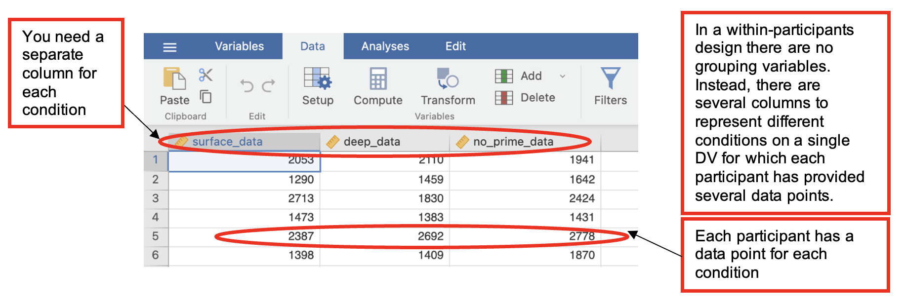
The hypotheses are (almost) the same as well but the data need to be entered differently into Jamovi, as in the next table. Each participant’s data must be entered on a single row, so where a participant provides three data points, these need to be entered next to each other along the same row.

Surface Priming RT (scale variable) [surface_data]	Deep Priming RT (scale variable) [deep_data]	No-Priming RT (scale variable) [no_prime_data]
Participant 1 data for surface	Participant 1 data for deep	Participant 1 data for no_prime
Participant 2 data for surface	Participant 2 data for deep	Participant 2 data for no_prime
Participant 3 data for surface	Participant 3 data for deep	Participant 3 data for no_prime

The hypotheses tested were:
- Participants will categorise words which they have previously processed at a deep level more quickly than words they have processed at a surface level or in the no prime condition.
- If surface processing has any effect on later categorization, the response times in the surface condition should be faster than in the no prime condition.

Walk-Through Example 1 “The effect of priming on a categorization task (repeated measures)”

Inspect the data

Download and open the RMC_NM1_1way_within_ANOVA.sav dataset from the Canvas folder.
Click on the “Data” tab and check the data looks something like below…

Check Parametric Assumptions

Go to Analyses -> Exploration -> Descriptives. In the dialog box, enter all repetitions of the DV into the ‘Variables’ box.
Go to ‘Plots’. Check ‘Histogram’ and ‘Box Plot’ Check whether the data are normally distributed (a parametric assumption that needs to be met for ANOVA).

In this example all the data are positively skewed. This is the usual pattern in response time data and there has been some controversy around how this should be dealt with when analysing such data.
For the purposes of Level 2 research methods, we will treat response time data as ‘approximately normal’ where the long tail of the distribution does not extend beyond 3 standard deviations above the mean.

Carry out the ANOVA

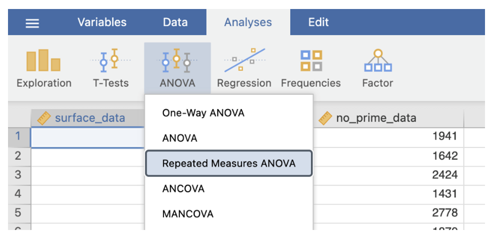
Go to Analyses -> ANOVA -> Repeated Measures ANOVA

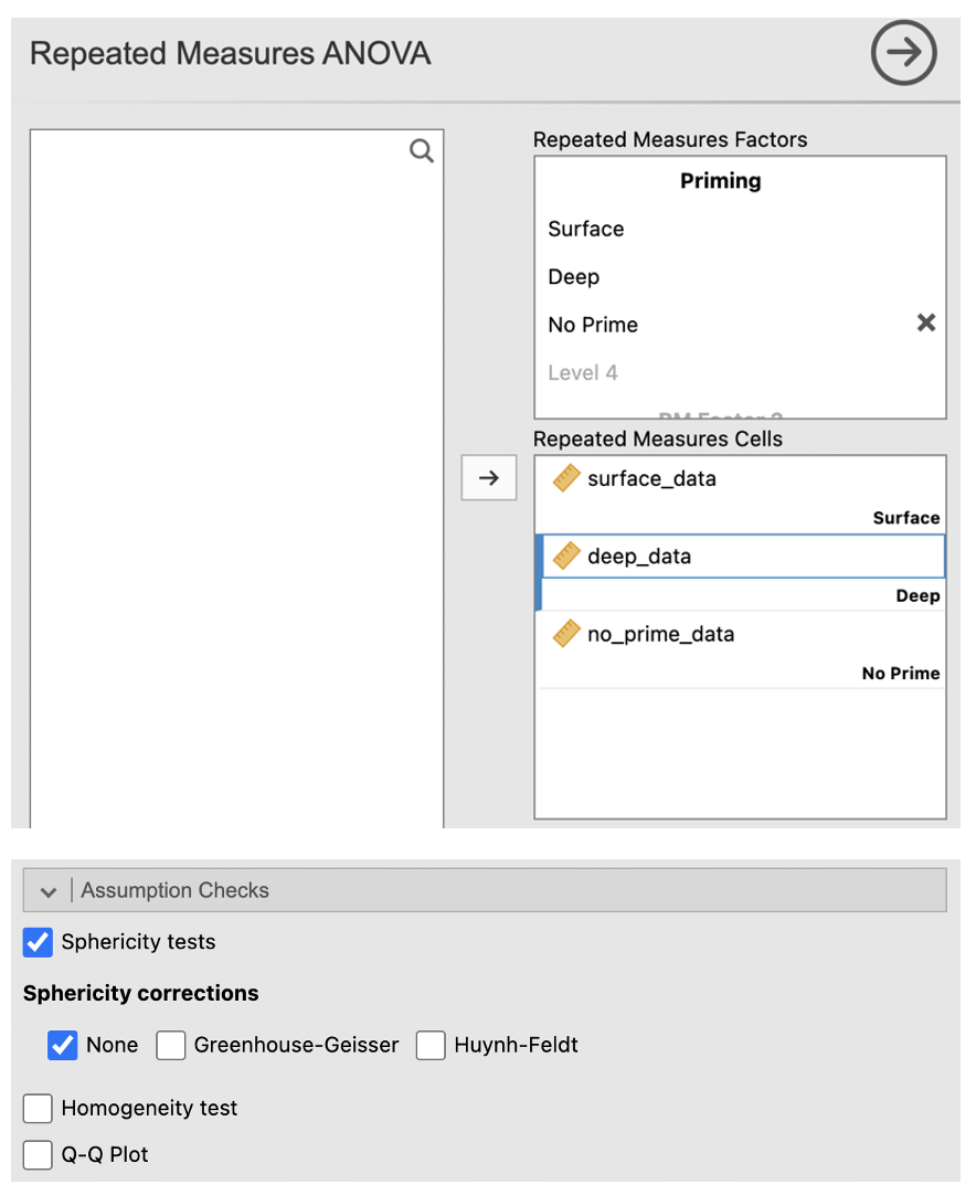
In the dialog box, enter a name for the IV into the ‘RM Factor 1’ box (e.g. “Priming”). Change the name ‘Level 1’ to the name of the first condition. Continue with the other 2 conditions (change ‘Level 2’ to the second and change ‘Level 3’ into the third).
Move the conditions into their respective cells in the ‘Repeated Measures Cells’ box.
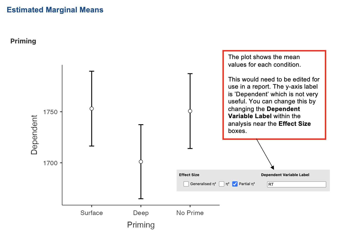
Click the box ‘Partial η2’ under Effect Size.
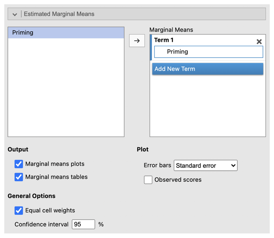
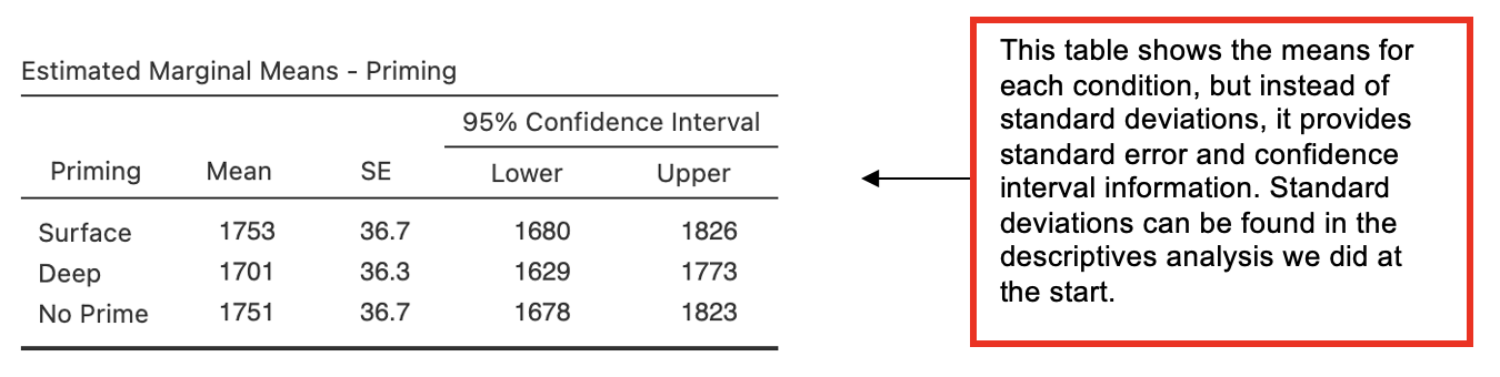
Go to ‘Estimated Marginal Means’. Enter the IV into the ‘Term 1’ box. Select ‘Marginal mean table’.
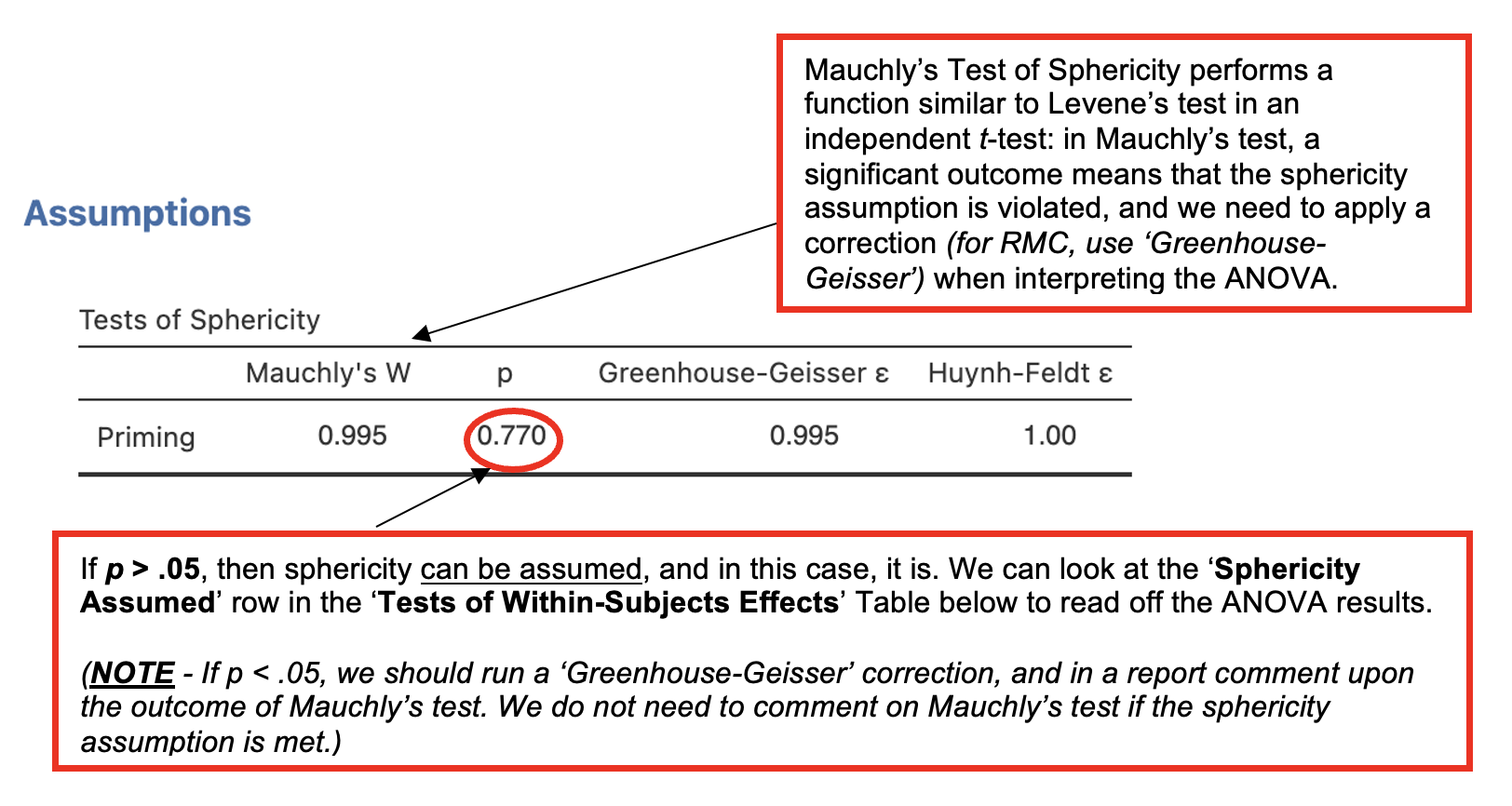
Go to ‘Assumption Checks’ and check ‘Sphericity tests’

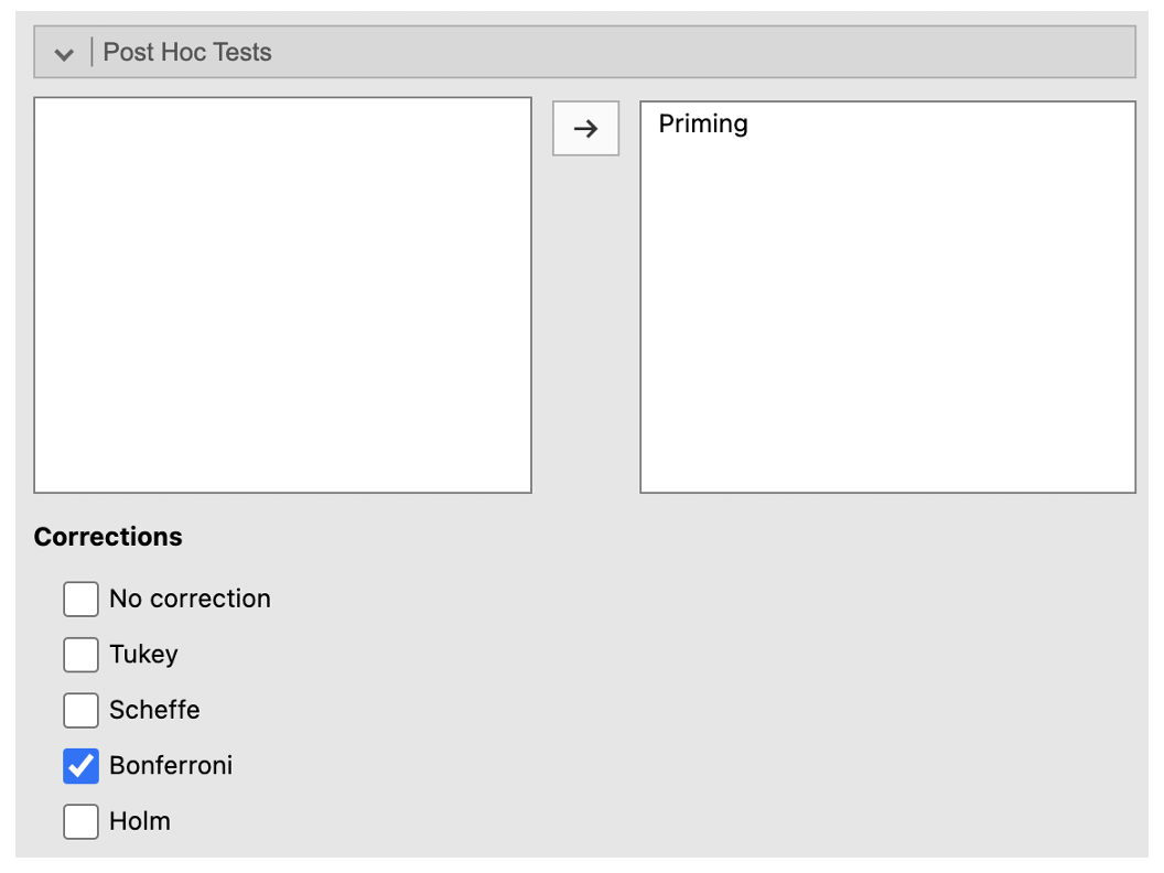
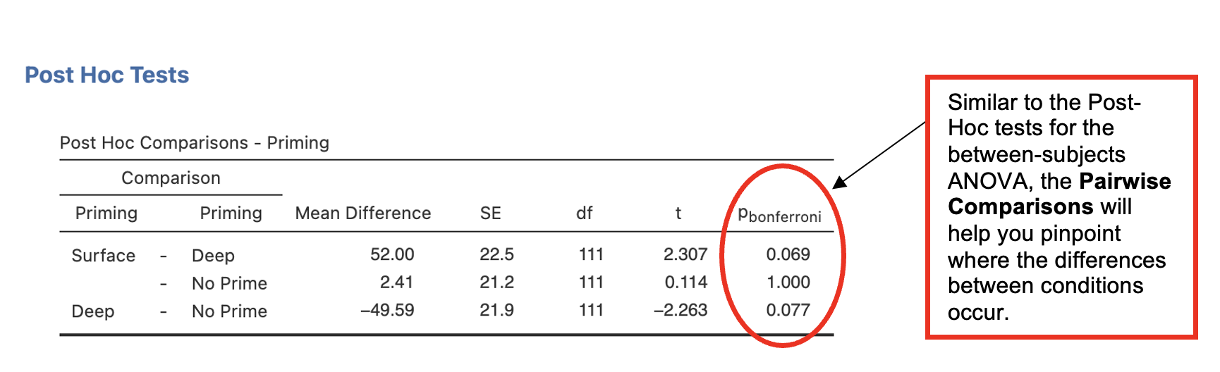
Got to ‘Post Hoc Tests’. Place ‘Priming’ into the right-side box. Check ‘Bonferroni’ under Corrections.

Jamovi output: One-way Repeated Measures ANOVA

Jamovi Output One-way ANOVA (within) questions

Question 1

Which (if any) condition(s) is significantly different from “no prime”?

Which (if any) condition(s) is significantly different from “deep”?

Writing up the ANOVA

One-way ANOVA (within) Write Up

Fill in the blanks

(Any data preparation, e.g. how the response times were calculated or how the data were trimmed or if and how many outliers were removed, should be presented in the section of the method about data preparation and data analysis.)

In a report, an ANOVA results section could look like this:

Results

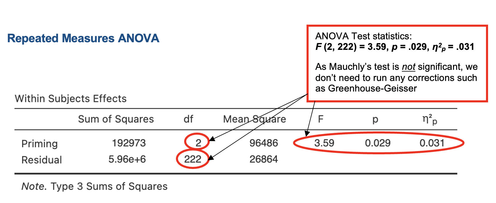
Although the mean categorization times were lowest in the deep priming condition as predicted, the categorization times in the no priming condition were very similar to those in the surface priming condition. A one-way repeated measures ANOVA found a small but significant effect of priming condition on categorization times (see Table 1).

Table 1 Means (Standard Deviations in Parentheses), and One-Way Analysis of Variance Statistics for Categorization Times (ms) for the Priming Conditions.

Measure		Priming Condition		F(2,[])	η²_p
	Surface	Deep	No-prime
Categorisation time	(388)	1701 (384)	1751 ()	3.6*	.03

*p <0.05

Using Bonferroni-corrected pairwise comparisons to carry out post-hoc analyses, none of the difference between the conditions were found to be significant. The difference between the surface priming and conditions (mean difference = ms, p = ) came closest to significance. The difference between and no priming (mean difference = 50ms, p = .077) also approached significance. There was no significant difference between surface and conditions. These findings the hypothesis.

2. Comparing more than 2 conditions when parametric assumptions are not met

If the data do not meet parametric assumptions, we should take a more conservative approach to avoid making errors in the conclusions we draw.
When we are dealing with data that are strongly skewed and/or have unequal variances, we should perform non-parametric tests to explore our effects. Non-parametric tests are also useful for ordinal data, as they work with ranks rather than absolute values.

Non-parametric equivalents

Most of the tests you have covered so far have a direct non-parametric equivalent. The table below shows how they map:

Parametric Test	Non-Parametric Equivalent
Pearson’s correlation*	Spearman’s correlation*
Independent samples t-test	Mann-Whitney
Paired samples t-test	Wilcoxon
Between-participants one-way ANOVA	Kruskal-Wallis
Repeated-measures one-way ANOVA	Friedman

*More on correlations in RMD

Kruskal-Wallis – Non-Parametric Comparison of More Than Two Independent Groups

For a one-way ANOVA design with more than two independent groups, where the data do not meet parametric assumptions, we can use the Kruskal-Wallis test. We might also use this with very small or unequal sample sizes.
In this example, we want to know whether the day of the week (Monday, Tuesday, Thursday, or Friday) on which a group of students attends workshops for a research methods module affects how much they look forward to the module (rated on a 5-point scale).
The hypothesis tested was:
- There are differences in self-rated looking forward score for taking part in the research methods module depending on the day of the week on which participants attend the workshop.
  - Note – this is a two-sided hypothesis as no direction for the effect of day of attendance is specified.

Walk-Through Example 2 “The effect of day of the week on looking forward to a research methods module.”

Download and open the RMC_NM1_lookfwd_Kruskal-Wallis.sav dataset
Click Analyses -> Exploration -> Descriptives. In the dialog box, enter the DV into the ‘Variables’ box. Enter the IV into the ‘Split by’ box.
Go to ‘Plots’. Check ‘Histograms’.

Record the medians and minimum and maximum scores from the Explore output [which is not presented here].

Measure				Day of the Week
	Monday		Tuesday		Thursday		Friday
	Mdn	Min-Max	Mdn	Min-Max	Mdn	Min-Max	Mdn	Min-Max
Looking forward score	3.0	2-4	3.0	2-3	4.0	3-4	3.0	1-3

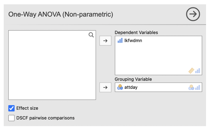
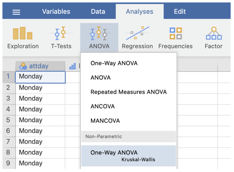
Go to Analyses -> ANOVA -> One-Way ANOVA Kruskal-Wallis (under non-parametric)
Enter the DV into the ‘Dependent Variables’ box. Enter the between-participants factor into the ‘Grouping Variable’ box
Tick the ‘Effect size’ box

Jamovi output: Kruskal-Wallis Test

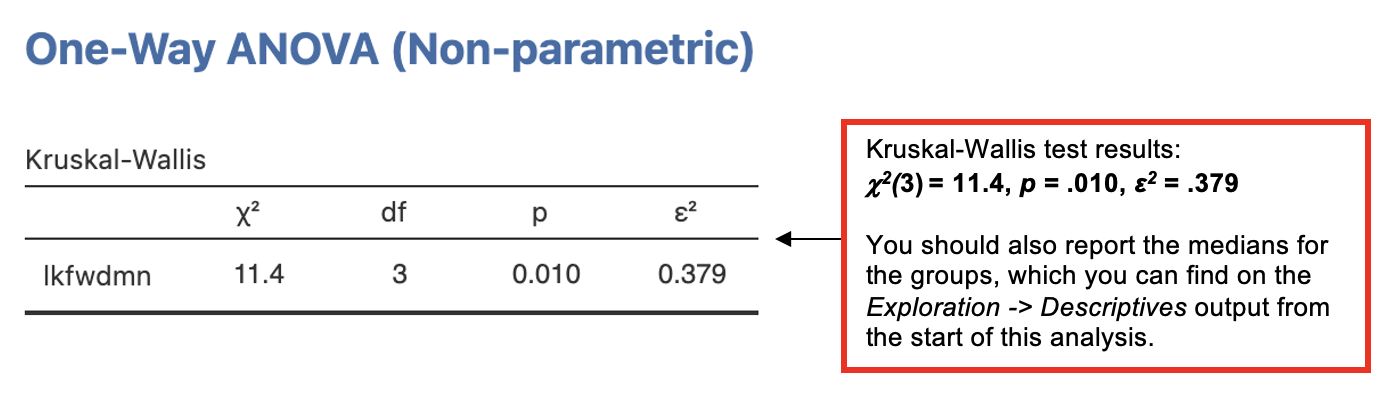
Since the Kruskal-Wallis test is significant, we need to follow it up with a post-hoc test to determine where the significant differences between the groups occur.
We could do this by performing Mann-Whitney tests (non-parametric comparison between two independent groups) to compare the different groups (levels) of the IV.
- To avoid family-wise error, adjust the significance level depending on the number of paired comparisons performed using Bonferroni’s correction.
- The correction is worked out by dividing the p-value acceptable for significance by the number of comparisons to be performed:
  - E.g. if we accept p < .05 as a cut-off for significance, then for 4 comparisons, the Bonferroni adjusted p-value =.05 / 4 = .0125. This means that any p-value greater than .0125 would not be considered significant.
However, there is no simple way of doing this on Jamovi, unless you create new data sheets (or new variables) with only two subgroups included for each analysis.
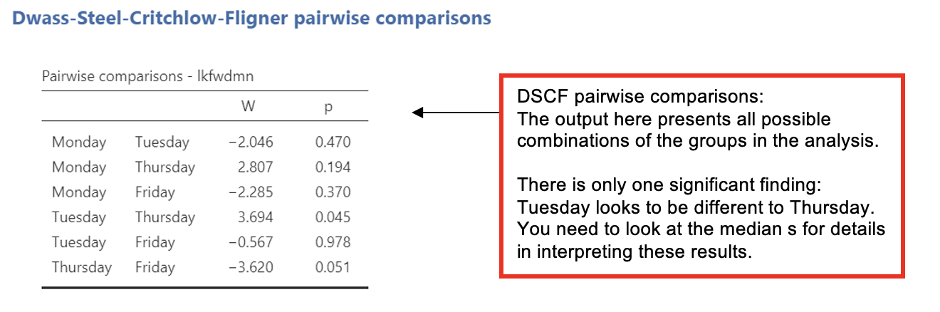
Jamovi offers an option for pairwise comparisons called the ‘Dwass-Steel-Crithclow-Fligner pairwise comparions’ or ‘DSCF pairwise comparisons’. There’s a box you can select when running the Kruskal-Wallis test.
- This test is two-sided and provides protection for family-wise error rates, like the Bonferroni correction does.

Reminder

We need to look up the medians and minimum and maximum values for each condition from the Exploration analysis and report those.

Jamovi output Kruskal-Wallis Test Post-Hoc

Writing up a Kruskal-Wallis Test

Kruskal-Wallis Write Up

Fill in the blanks

In a report, a Kruskal-Wallis results section could look like this:

Results

Because the participant numbers were small and unequal across conditions and the score for how much participants looked forward to the module was ordinal and not normally distributed, a Kruskal-Wallis test was performed to examine the effect of day of the week upon the mean look-forward score (out of 5). It was found that day of the week had a significant effect on look-forward ratings, chi-sq²(3) = , p = , ε2 = .379.

Table 1 shows the median look-forward scores for each day and paired comparisons (DSCF pairwise comparisons). Only the difference between look-forward scores for Tuesday compared with was statistically significant. The hypothesis that the day of study affects how much students look forward to their research methods module was .

Table 1 Median look forward scores (out of 5) by day of the week and including significance of paired comparisons.

Day	Median look forward score	Paired comparison significance
		Monday	Tuesday	Thursday	Friday
Monday		-	-	-	-
Tuesday	3	p - .470	-	-	-
Thursday		p - .194	p - .045*	-	-
Friday	3	p - .370	p - .978	p - .051	-

*p <0.05

Friedman Test – Non-Parametric Comparison of More Than Two Repeated Measures

With a related (within-participants or repeated measures) design, where the data are non-parametric, we can use the non-parametric equivalent of the repeated measures one-way ANOVA: the Friedman test.
In this example, we test if there is a difference in how much the group of students from the previous example looks forward to their workshops on the research methods module (rated on a 5-point scale) depending on how long they have been attending the module (at the start, after 2 weeks, after 5 weeks).
The hypothesis tested was:
- There are differences in self-rated looking forward score for taking part in the research methods module depending on how long the participants have been attending the workshops.

Walk-Through Example 3 “The effect of length of attendance on looking forward to a module”

Download and open the RMC_NM1_lookfwd_Friedman.sav dataset
Go to Analyses -> Exploration -> Descriptives. In the dialog box, enter all repetitions of the DV into the ‘Variables’ box.
Go to ‘Plots’. Check ‘Histograms’.

Record the medians and other key descriptive statistics (e.g. maximum and minimum scores) from the Explore output [which is not presented here].

Measure		Time spent studying the module
	At Start		After 2 Weeks		After 5 Weeks
	Mdn	Min-Max	Mdn	Min-Max	Mdn	Min-Max
Looking forward score	3.0	2-5	3.0	1-4	3.0	1-4

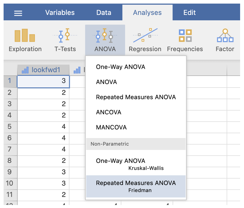
Go to Analyses -> ANOVA -> Repeated Measures ANOVA Friedman (under non-parametric)
Enter all levels of the DV into the ‘Measures’ box

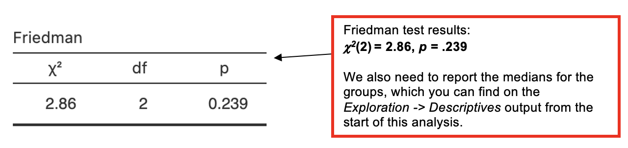
Jamovi output: Friedman Test

Since the Friedman test is not significant, we do not need to carry out a post-hoc analysis.
If we did need to carry out post-hocs, we would use Wilcoxon tests (non-parametric comparison between two related conditions) to compare pairs of conditions.
- To avoid family-wise error, adjust the significance level depending on the number of paired comparisons performed using Bonferroni’s correction, i.e. divide the p-value acceptable for significance by the number of comparisons to be performed:
  - E.g. for 3 comparisons, the Bonferroni adjusted p-value = 0.05 / 3 = 0.0167.
- This is can be done easily on Jamovi. It should look something like this.

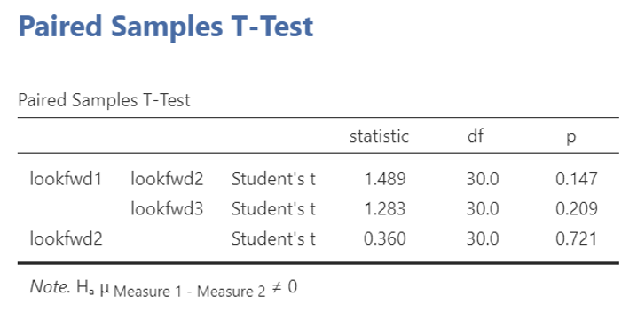
Jamovi output: Friedman Test post-hocs using Wilcoxon and a Bonferroni correction

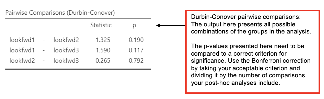
Alternatively, the Friedman test dialogue on Jamovi also offers Durbin-Conover Pairwise Comparisons, however, this test does not correct for family-wise error.
- If you use Durbin-Conover comparisons, you should use a correction against the p-value you use for the comparisons.
  - E.g. for 3 comparisons, the Bonferroni adjusted p-value = 0.05 / 3 = 0.0167.
  - In a results section, state that you used the Bonferroni correction and what the new criterion for significance was against which you compare the individual p-values for the comparisons.

Jamovi output: Friedman Test post-hocs using Wilcoxon and a Bonferroni correction

Reminder

We need to look up the medians and minimum and maximum values for each condition from the Exploration analysis and report those.

Writing up a Friedman Test

Friedman Write Up

Fill in the blanks

In a report, a Friedman results section could look like this*:

Results

Histograms for the three conditions were inspected separately. As the data were skewed and the look forward scores were measured on an ordinal scale, a Friedman test was used. There was no significant effect of time spent studying the module upon look forward scores, chi-sq²() = 2.86, p = . In fact, the median score for all three conditions was identical at , and the hypothesis that time spent studying on the module would affect how much people looked forward to the workshop sessions was .

*Note that the post-hocs are not reported here, as the main analysis was non-significant.

NOTE

Download and open the RMC_NM1_SPSS_attitude.sav dataset and answer the following questions. Before you start, recode the marks data into a new grouping variable called “grade_class” so that participants are allocated to either first_class (70-100), upper_second (60-69) or lower_second_or_below (0-59) groups.

Activity Questions

Which type of statistical analysis would you need to carry out to test the hypothesis that “People with first class grades, upper second class grades, and lower second class or below grades on the first practical vary on their total score for the attitudes towards SPSS* (where a high score indicates a positive attitude towards SPSS)”?

Think about you reasoning for choosing this test before looking at the question 1 notes.

*This is the stats package we taught before we shifted to teaching Jamovi.

The wording of the hypothesis suggests that there are different groups of people being studied. This means that an independent (between-participants) design was being used.

There is a single factor which could be called grade-class or something similar. This means that the design is a one-way design.

If you Explore the data using SPSS, you can see that the data on the SPSS attitudes (the DV) are normally distributed - either if you look at the DV as a whole or if you look at the different grade-range groups.

Sample sizes are also similar and the range of variation in each group is similar.

Based on this consideration, it is appropriate to us an ANOVA to test the hypothesis.

A Kruskal-Wallis analysis would also be correct, if parametric assumptions are not met.

Using the appropriate walk-through example (from Workshops 2 or 3), carry out this test and inspect the output. How many participants are there in the “lower_second_or_below” group?

N =

What is the mean score and standard deviation for the “first_class” group?

Mean =

SD =

What is the appropriate test statistic (including the appropriate degrees of freedom)? What was the value of the test statistic (if it is a Greek letter type the name e.g. ‘chi-square’) and what was the associated p-value?

Test statistic = ; p =

What was the measure of effect size (type its name, e.g. ‘partial eta squared’ or ‘epsilon squared’) and what was the value of the effect size?

Effect size =

If the test was significant, between which groups do the significant differences occur?