Week 4 : Factorial ANOVA with Jamovi

Learning Objectives

	Quantitative Methods
	Understand and interpret ANOVA outputs

	Data Skills
	Two-way between-participants ANOVA
	Two-way repeated measures ANOVA
	Two-way mixed ANOVA

	Open Science
	Working with openly available research data

NoteToday’s session

In today’s session we will explore more complicated ANOVA designs. The real power of ANOVA is that it allows us to examine interactions between two or more variables so we can examine how different factor combinations affect our participants.

• There are three ways in which we can set up a study to explore two factors with two levels each:

  1. A different group of participants takes part in each condition (independent/between-participants 2x2 design).
  2. The same group of participants takes part in all conditions (repeated measures/within-participants 2x2 design).
  3. Two different groups of participants take part in two conditions each (mixed 2x2 design).

• In lectures and computer practicals, we will also talk about how:

  • A factorial ANOVA can have more than two conditions on each of its factors – just as a one-way ANOVA has three or more conditions on one factor.

    1. E.g. a two-way ANOVA might have one factor with three conditions and one with four. This would be called a ‘3x4’ design.
    2. If a factor with more than 2 conditions has a significant main effect, we need to follow up using a post-hoc comparison as we would do for a one-way ANOVA.

• A factorial ANOVA can have more than two factors. This means that there are more interactions to consider and interpret. Usually our research questions and hypotheses play an important role in interpreting these interactions.

  1. E.g. a three-way ANOVA might have three factors with two conditions each – this is called a ‘2x2x2’ design.

  2. Designs can be extended by using more conditions (e.g. 2x2x3 designs) or by adding more factors (e.g. 2x2x2x2 designs). The same principles apply:

     1. If there are more than two conditions and a significant effect, a post-hoc is needed to identify which conditions are different to each other.
     2. If there more factors, there will be more interactions to interpret.

1. Two between-participants IVs: 2x2 independent ANOVA

• In this example, we want to test if using the word “certain”, with either “It is” or “I am” as a prefix, influences someone’s decision making (whether they intend to make a bet). This factor is called communication mode, with two levels: internal (“I am”) vs. external (“It is”).

• We also want to test if the speaker’s expertise (novice vs. expert) affects intention to bet and if expertise interacts with the effect of the communication mode.

• Hypotheses:

  1. We predict that internal mode of communication will have a greater influence on intention to bet than external mode of communication, and that a recommendation from an expert will have a greater effect upon intention to bet than a recommendation from a novice.

  2. We expect this difference between experts and novices to be particularly pronounced for the internal mode of communication, such that an expert saying ‘I am certain’ will be particularly influential for intention to bet. [<- this part predicts an interaction.]

• Different participants should take part in each condition of this experiment to avoid confounding of decision-making from previous experiences with the task.

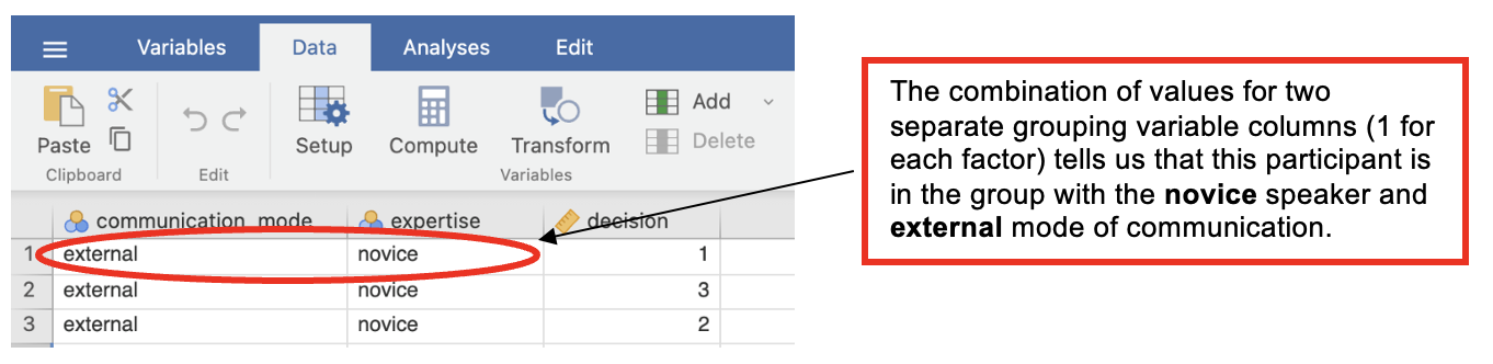
• The data need to be entered like this on Jamovi:

Communication mode (nominal variable with values 1 and 2) [grouping variable 1]	Expertise (nominal variable with values 0 and 1) [grouping variable 2]	Intention to bet (scale variable; for intention to bet, each participant’s individual score is recorded)
1 (where 1 = external)	0 (where 0 = novice)	Data for group 1. Each row has the same value for communication mode (i.e. 1) and for expertise (i.e. 0)
1 (where 1 = external)	1 (where 1 = expert)	Data for group 2. Each row has the same value for communication mode (i.e. 1) and for expertise (i.e. 1)
2 (where 2 = internal)	0 (where 0 = novice)	Data for group 3. Each row has the same value for communication mode (i.e. 2) and for expertise (i.e. 0)
2 (where 2 = internal)	1 (where 1 = expert)	Data for group 4. Each row has the same value for communication mode (i.e. 2) and for expertise (i.e. 1)

Walk-Through Example 9 “The effects of communication mode and speaker expertise upon intention to bet”

Inspect the Data

1. Download and open the RMC_NM1_uncertainties_2x2_between.sav dataset
2. With two independent factors, you need two grouping variables, one for each factor, and a scale variable for the DV. The condition a participant took part in is determined by the combination of the two grouping variables.

Check Parametric Assumptions

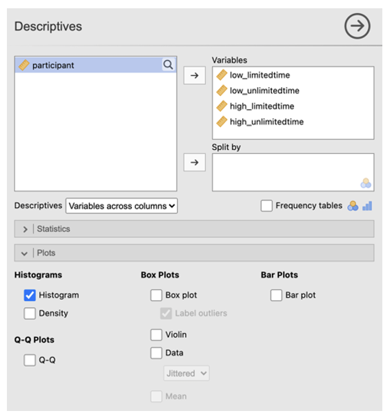
3. Go to Analyses -> Exploration -> Descriptives
4. In the dialog box, enter the DV into the ‘Variables’ box. Enter all IVs into the ‘Split by’ box. Go to ‘Plots’. Check ‘Histograms’.

NoteNote

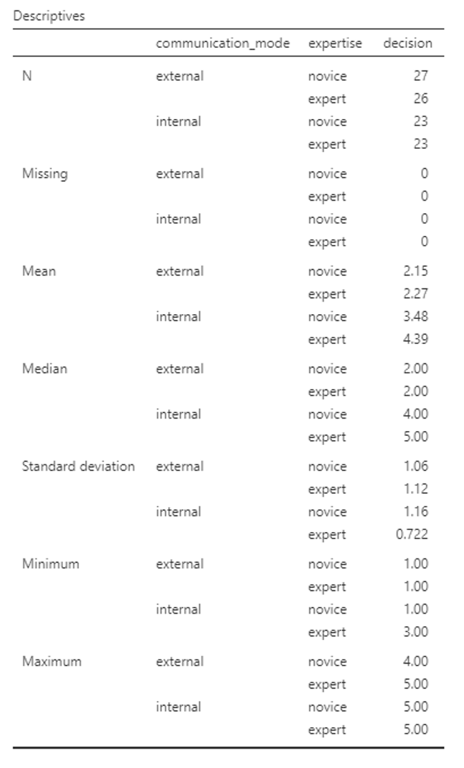
In this analysis, the individual conditions are skewed. This is in part due to the DV being measured on a very restricted scale (out of 5). However, all four conditions are showing some variability. So given that there is no non-parametric equivalent for 2 x 2 ANOVA, we would still run the ANOVA here.

Descriptive Statistics

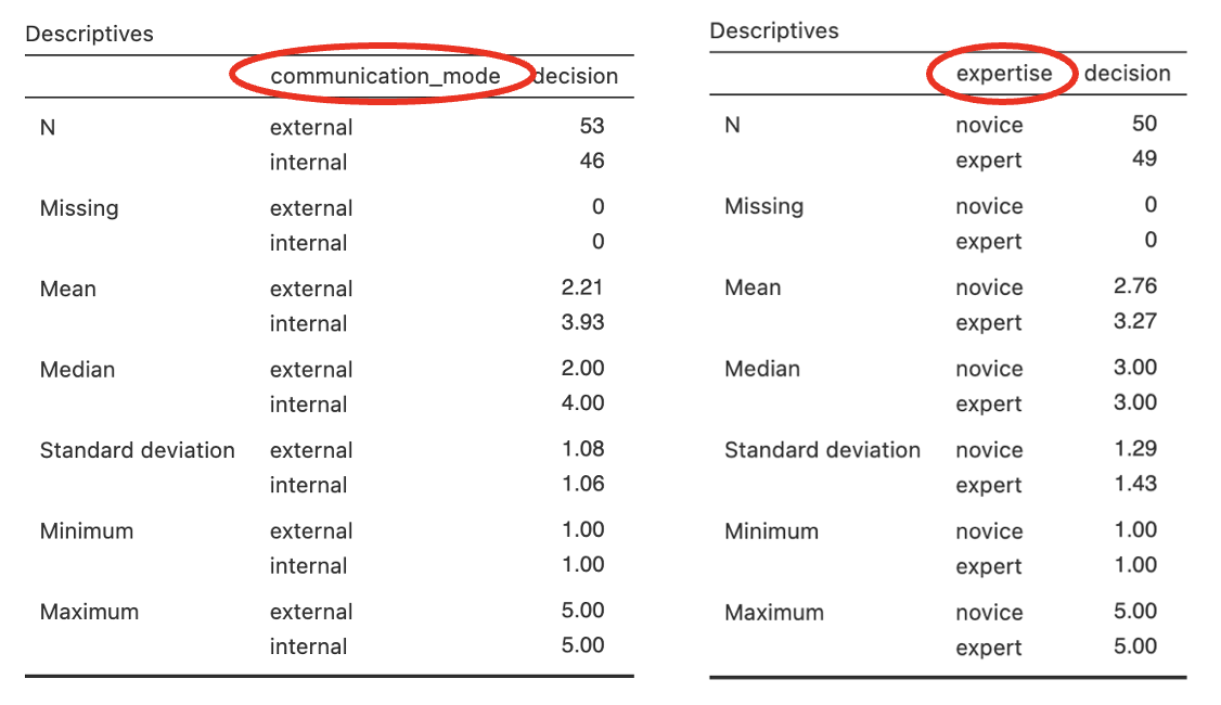
5. To get the descriptive statistics for the main effects in Jamovi you need to run the analysis separately.

6. Go to Analyses -> Exploration -> Descriptives

7. In the dialogue box, enter the DV into the ‘Variables’ box. Enter the IVs into the ‘Split By’ box.

If you want to calculate the means for each IV separately, do this: In the dialogue box, enter the DV into the ‘Variables’ box. Enter just one IV into the ‘Split By’ box. Repeat steps f and g for the other IV.

Carry out the ANOVA

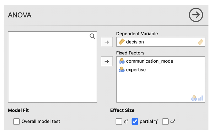
8. Go to Analyses -> ANOVA -> ANOVA

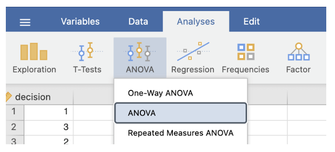
1. In the dialog box, enter the DV into the ‘Dependent Variable’ box. Enter the two IVs in the ‘Fixed Factors’ box.

10. Check the box next to ‘partial η²’

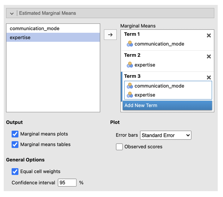
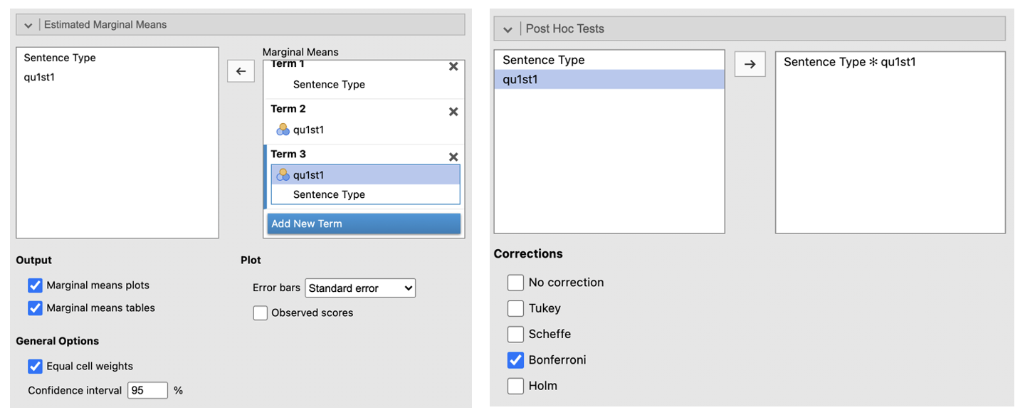
11. Go to ‘Estimated Marginal Means’. Enter the first IV in the Term 1 box. Click ‘Add New Term’. Enter the second IV into the Term 2 box. Click ‘Add New Term’. Enter the IV that you want to be displayed on the horizontal axis first in the Term 3 box (if one of your IVs is about time, e.g. ‘before’ and ‘after’ conditions, put this on the horizontal axis). Enter the IV you want to be displayed as separate lines second in the box Term 3 box. Change the error bars to ‘Standard Error’. Check the box next to ‘Marginal means plots’ and ‘Marginal means tables’.

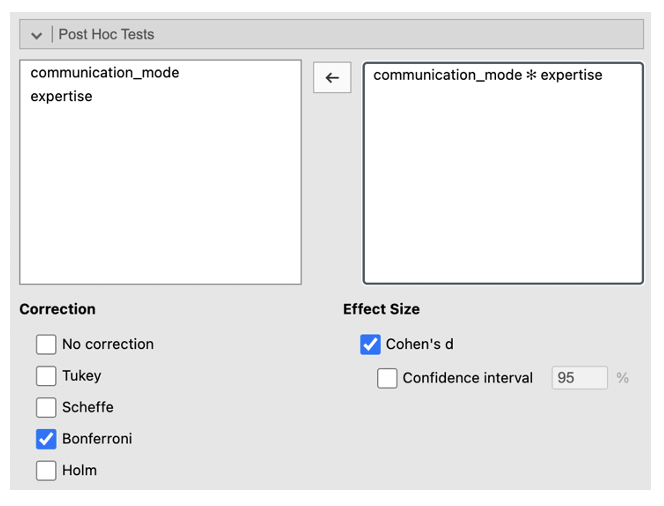
12. Go to ‘Post Hoc Tests’. Put the interaction into the box on the right. Select ‘Bonferroni’ from the Correction list. Check ‘Cohen’s d’ under Effect Size. This will allow you to identify where differences between conditions are, as with a one-way ANOVA.

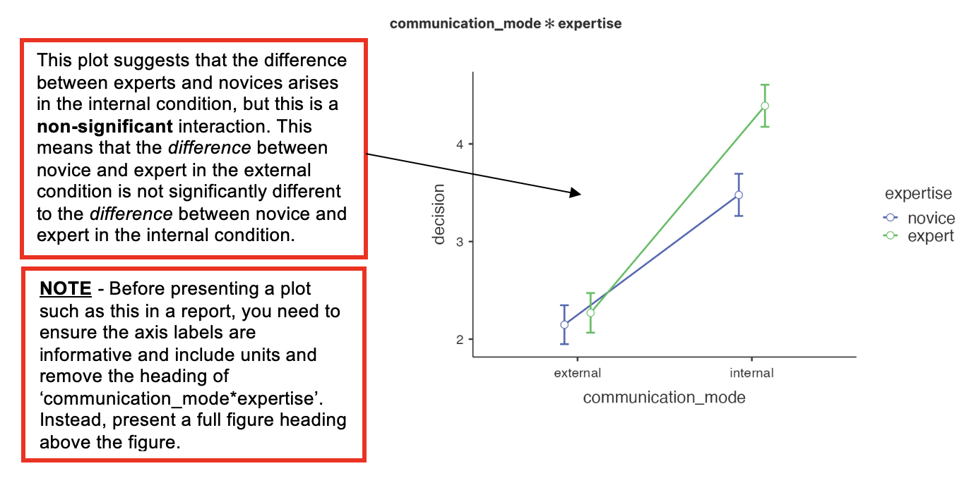
Jamovi output: 2x2 Independent ANOVA

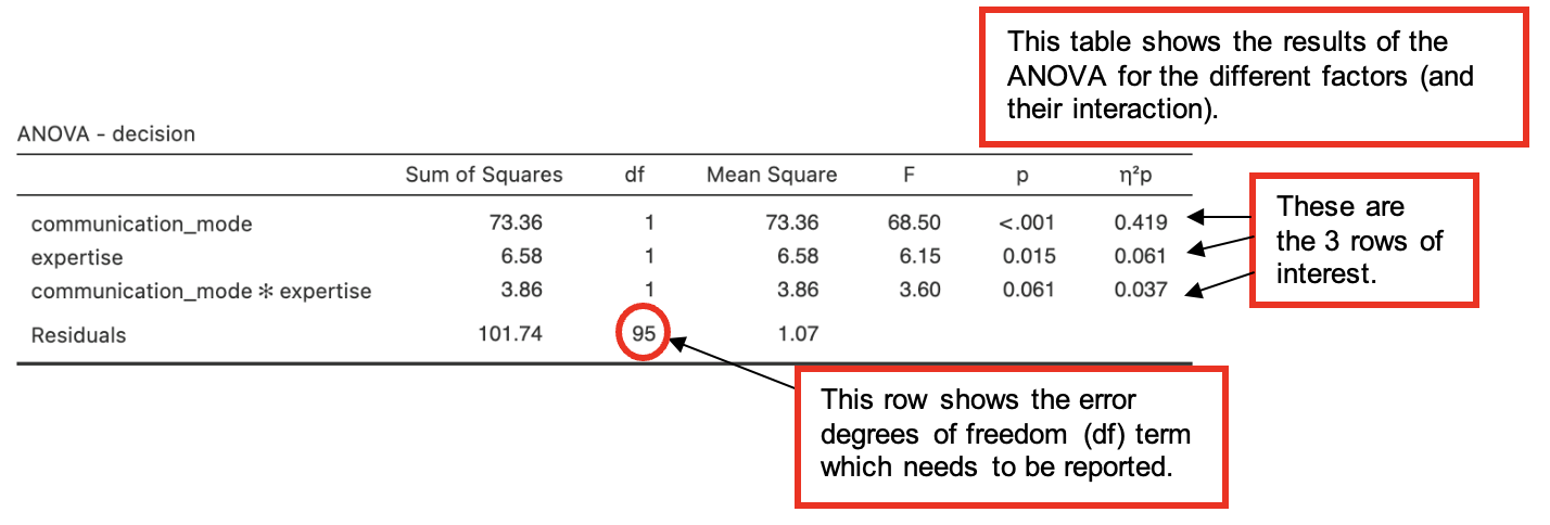
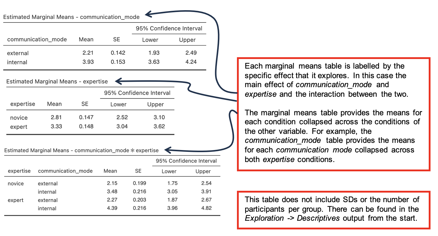
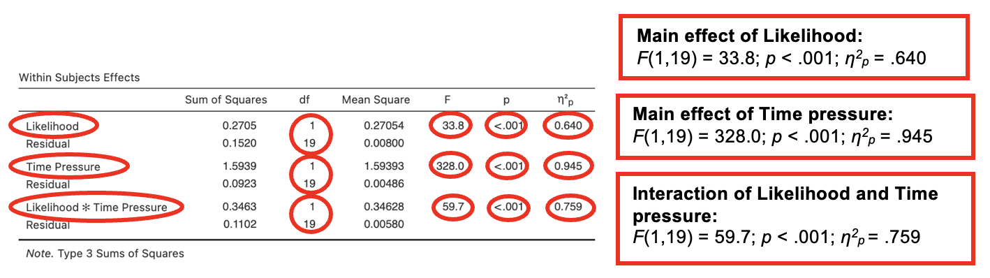
The three rows labelled “communication_mode”, “expertise” and **“communication_mode*expertise” are most important in interpreting this output. (We also need to look at the “Residuals”** row, for the error df term.)

1. The “communication_mode” row shows that there is a significant main effect of communication mode upon the intention to bet, F(1, 95) = 68.50, p < .001, η2p = .419.
   1. The estimated marginal means table for communication_mode provides information about the direction of the difference. Here intention to bet (decision) is greater for internal mode communications than for external mode.
   2. Partial eta squared (η²p) tell us that this effect explains 42% of the variance in the data. This is a medium to large effect size.
2. The “expertise” row shows that there is also a significant main effect of expertise upon the intention to bet, F(1, 95) = 6.15, p = .015, η2p = .061.
   1. See the estimated marginal means table for expertise for details of the difference. Here expert advice leads to a slightly higher intention to bet than novice advice.
   2. An effect size (η²p) of 6% is small. In terms of discussing the findings, this means that speaker expertise plays a less important role when considered on its own than communication mode.
3. Finally, the **“communication_mode*expertise” [pronounced ‘communication mode by expertise’] row shows that the interaction between communication mode and expertise is not significant, F(1, 95) = 3.60, p = .061, η2p = .037.** [Note – the effect size is not always reported when an effect is not significant.]
   1. As the interaction is nearly significant, we might comment on this in a report.

• If an interaction is significant, we would look at the interaction plot to examine it. Jamovi presents this near the end of the output, but looking at this before working through all the other tables Jamovi provides can be helpful for interpreting the findings.

Estimated Marginal Means tables

Post Hoc Comparisons Tables

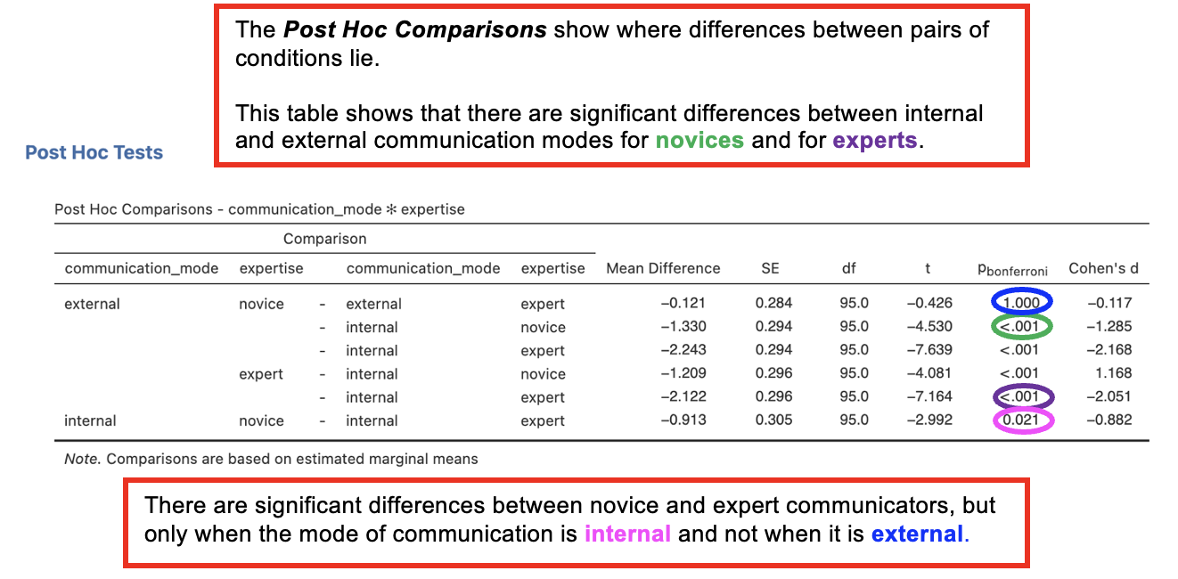
• The post hoc comparisons sections of the output explores the interaction by looking at differences in pairs of conditions, thus providing more detail about the nature of the observed effects
  • These tables show the results of t-tests between the different pairs of variables

Writing up 2x2 independent ANOVAs

Tip2x2 independent ANOVA Write Up

Fill in the blanks

(Any data preparation, e.g. how the response times were calculated or how the data were trimmed or if and how many outliers were removed, should be presented in the section of the method about data preparation and data analysis.)

In a report, an ANOVA results section could look like this:

Results

The intention to bet for each group was analysed using an independent 2 (communication mode: external vs. ) x 2 (level of expertise: vs. expert) analysis of variance. The ANOVA found significant main effects on intention to bet for communication mode, F(1, ) = , p < .001, η²p = , and for level of expertise, F (1, 95) = 6.15, p = , η²p = .061. The interaction between communication mode and level of expertise was approaching significance, F(1, 95) = , p = .061, η²p = .037.

The results broadly supported the hypothesis in that expert recommendations were more effective than novice ones, and across both levels of expertise the external mode of communication was less effective than internal mode.

Although the interaction effect did not reach significance, the results supportpartially supportdo not support the prediction that the effect of expertise would be particularly noticeable in the internal mode of communication (see Table 1).

Table 1. Mean intention to bet (out of 5) for external and internal communication mode depending on level of expertise of speaker (standard deviation in parentheses).

Communication mode	Level of expertise
	Novice	Expert
External	(1.06)	2.27 (1.12)
Internal	3.48 (1.16)	4.39 ()

2. Two within-participants IVs: 2x2 repeated measures ANOVA

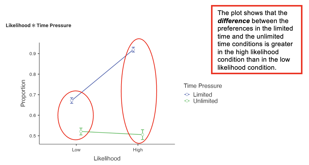
• In this example, we want to test if the preference for positive chance phrases (e.g., “it is likely”) over negative chance phrases (“there is little chance”) is affected by the likelihood of a described event (low chance vs high chance), and if this is in turn affected by the time pressure (limited time vs unlimited time) under which participants respond. The proportion of times that a participant indicated a preference for a positive chance phrase over a negative chance phrase was recorded.

• Hypothesis:

  • Preferences will be expressed more strongly when time is limited than when it is unlimited, and this effect will be particularly strong when likelihood of an event occurring is high.

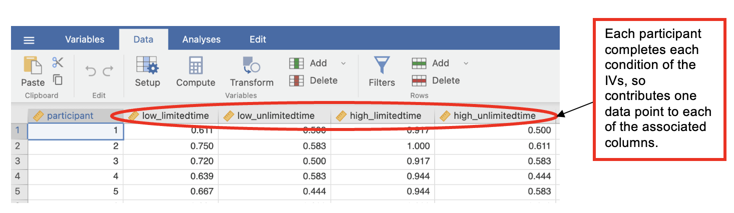
• To minimise error due to people’s individual differences, the same participants could take part in all conditions. The data need to be entered into Jamovi as follows:

Low likelihood, limited time (scale variable)	Low likelihood, unlimited time (scale variable)	High likelihood, limited time (scale variable)	High likelihood, unlimited time (scale variable)
Data for Cond. 1, Ppt 1	Data for Cond. 2, Ppt 1	Data for Cond. 3, Ppt 1	Data for Cond. 4, Ppt 1
Data for Cond. 1, Ppt 2	Data for Cond. 2, Ppt 2	Data for Cond. 3, Ppt 2	Data for Cond. 4, Ppt 2
Data for Cond. 1, Ppt 3	Data for Cond. 2, Ppt 3	Data for Cond. 3, Ppt 3	Data for Cond. 4, Ppt 3
…	…	…	…

NoteNote

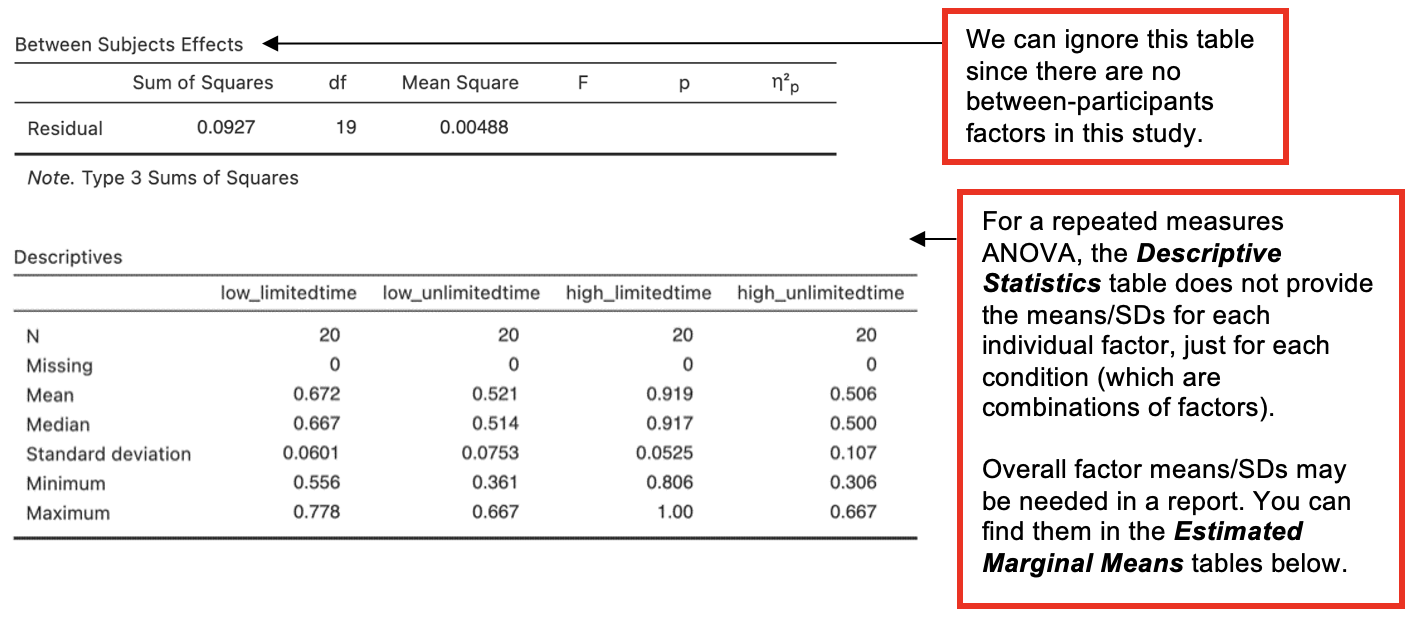
Although this looks like there are four DVs, this is not the case: only one thing was measured – the preference for positive phrases under four different circumstances. Notice that there is no grouping variable since all participants completed all of the different conditions and so were part of the same group.

Walk-Through Example 10 “The effects of likelihood and time pressure on preference for positive chance phrases”

Inspect the data

1. Download and open the RMC_NM1_directionality_2x2_within.sav dataset
2. With a repeated measures design, you do not have grouping variables, but you need 1 column for each data point you collect from the same participant.
   1. In a 2x2 repeated measures design that means 4 columns, 1 for each condition.

Check Parametric Assumptions

3. Go to Analyses -> Exploration -> Descriptives
4. In the dialog box, enter all columns of the DV into the ‘Variables’ box. Go to ‘Plots’. Check ‘Histogram’.

Carry out the ANOVA

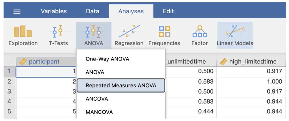
5. Go to Analyses -> ANOVA -> Repeated Measures ANOVA

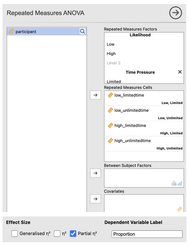
6. In the RM Factor 1 box, type a meaningful name for the first IV. Fill in the boxes with meaningful labels for the levels. e.g. ‘Likelihood’ for the IV overall, and ‘Low’ and ‘High’ for the levels of the IV.

7. In the RM Factor 2 box, type a meaningful name for the second IV. Fill in the boxes with meaningful labels for the levels. e.g. ‘Time Pressure’ for the IV overall, and ‘Limited’ and ‘Unlimited’ for the levels of the IV.

8. Add the variables in the correct ‘Repeated Measures Cells’ (match up the names of your columns with the labels in each cell. Check that the combinations are correct.

9. Check the box next to ‘partial η²’ under Effect Size and change the Dependent Variable Label to something meaningful. e.g. ‘Proportion’.

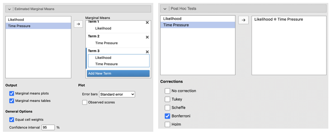
10. Go to ‘Estimated Marginal Means’. Enter the first IV in the Term 1 box. Click ‘Add New Term’. Enter the second IV into the Term 2 box. Click ‘Add New Term’. Enter the IV that you want to be displayed on the horizontal axis first in the Term 3 box (if one of your IVs is about time, e.g. ‘before’ and ‘after’ conditions, put this on the horizontal axis). Enter the IV you want to be displayed as separate lines second in the box Term 3 box. Change the error bars to ‘Standard Error’. Check the box next to ‘Marginal means plots’ and ‘Marginal means tables’.

11. Go to ‘Post Hoc Tests’. Put the interaction into the box on the right. Select ‘Bonferroni’ from the Correction list.

Jamovi output: 2x2 repeated measures ANOVA

Estimated Marginal Means tables on the Jamovi output

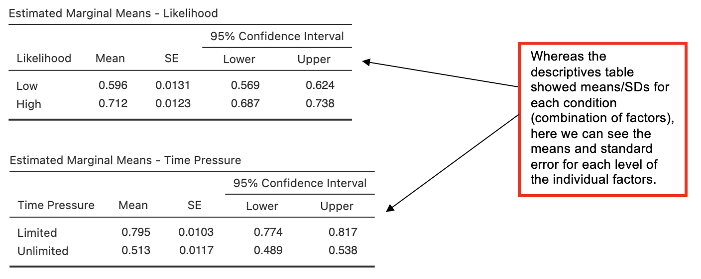
From the next part of the output, only the most relevant tables are reproduced here: the estimated marginal means for likelihood and for time_pressure.

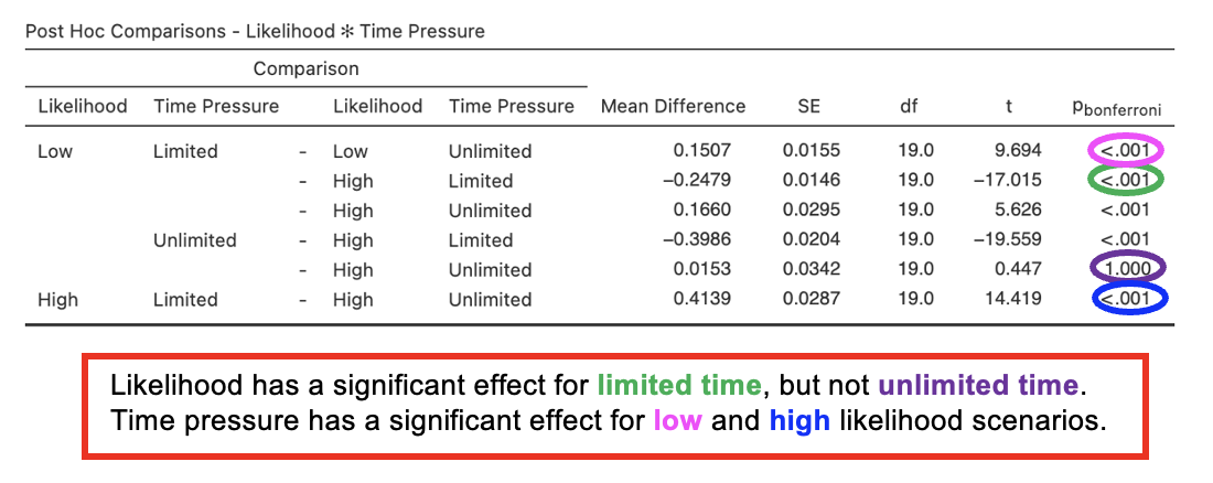
Post Hoc Comparison Tables

Interaction Plot

Writing up 2x2 repeated measures ANOVAs

Tip2x2 repeated measures ANOVA Write Up

Fill in the blanks

(Any data preparation, e.g. how the response times were calculated or how the data were trimmed or if and how many outliers were removed, should be presented in the section of the method about data preparation and data analysis.)

In a report, an ANOVA results section could look like this:

Results

The effects of likelihood (low vs. high) and time pressure (limited time vs. unlimited time) upon preference for positive chance phrases expressed as a proportion was tested with a 2x2 repeated measures ANOVA. As predicted there was a significant main effect of likelihood, F(1,19) = 33.8; p < .001; η²p = , and a significant main effect of time pressure, F(1,19) = ; p ; η²p = .945. The interaction between likelihood and time pressure was also significant, F(, ) = 59.7; p < .001; η²p = .

Preferences for positive chance phrases were expressed less strongly for low likelihood scenarios compared to high likelihood, while time pressure led to more strongly expressed preferences than when time was unlimited. In keeping with predictions, the interaction showed that the effect of time pressure was particularly strong for high likelihood scenarios compared to low likelihood scenarios (see Table 1).

Table 1. Mean preference for positive chance phrases (as a proportion) depending on likelihood of scenario and time pressure (standard deviation in parentheses).

Likelihood of scenario	Time allowed
	Limited	Unlimited
Low	.67 ()	.52 (0.08)
High	(.05)	.51 ()

(Report values to 2 d.p.)

3. One between-participants IV and one within-participants IV: 2x2 mixed ANOVA

• In this example, an experiment was conducted to look at the effect of sentence type (question vs. statement-to-verify) on the rate of semantic illusions.

• Since all participants are taking part in both conditions – they see question stimuli and statement stimuli, the order in which the sentence types are processed has been counterbalanced. We can therefore also look at whether presentation order (questions first or statements first) affects the rate of semantic illusions.

• The sentence type is therefore the within-participants (repeated measures) factor, and the presentation order is the between-participants factor in this design.

• Hypothesis:

  • Questions will lead to a higher semantic illusion rate than statements, regardless of presentation order.

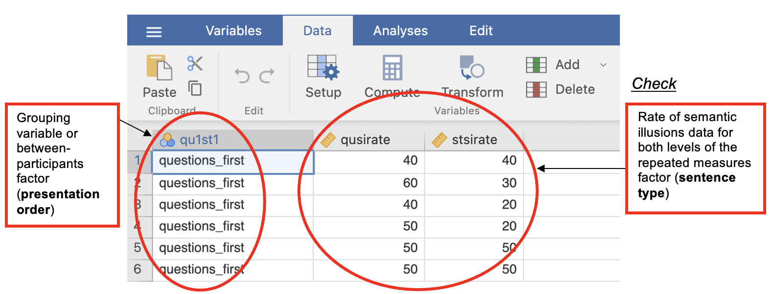
• The data for a mixed design need to be entered into Jamovi like this:

Order (qu1st1) (a nominal variable with values 1 and 2) [grouping variable 1]	Rate of semantic illusions with questions (qusirate) (scale variable)	Rate of semantic illusions with statements (stsirate) (scale variable)
1 (where 1 = questions first)	qusirate for Ppt 1 who saw questions first	stsirate for Ppt 1 who saw questions first
	qusirate for Ppt 2 who saw questions first	stsirate for Ppt 2 who saw questions first
	…	…
2 (where 2 = statements first)	qusirate for Ppt 1 who saw statements first	stsirate for Ppt 1 who saw statements first
	qusirate for Ppt 2 who saw statements first	stsirate for Ppt 2 who saw statements first
	…	…

Walk-Through Example 11 “The effects sentence type and presentation order upon semantic illusion rate”

Inspect the Data

1. Download and open the RMC_NM1_statements-questions_2x2_mixed.sav dataset
2. With a mixed design, you need one grouping variable and you need one column for each data point you collected from the same participant (or each level of the within-participants factor).
3. In a 2x2 mixed design that means three columns, one for each condition on the within-participants (repeated) measure and one for the grouping variable.

Parametric Assumptions

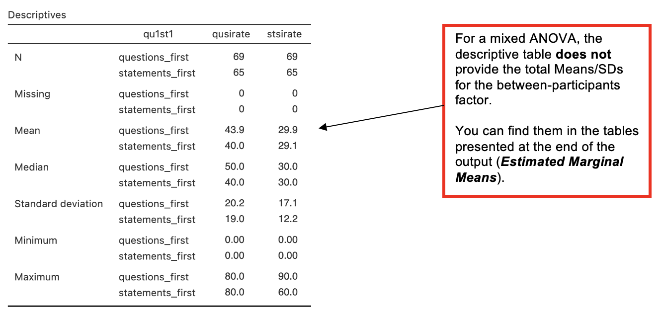
4. Descriptive Statistics. Go to Analyses -> Exploration -> Descriptives. In the dialog box, enter the two DVs (repeated measures) into the ‘Variables’ box.
5. Enter the grouping variable (between-participants IV) into the ‘Split By’ box. Go to ‘Plots’. Check ‘Histogram’.

Carry out the ANOVA

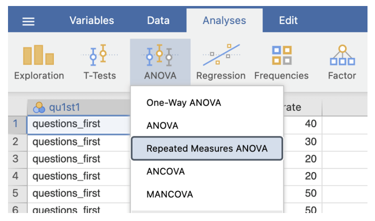
6. Go to Analyses -> ANOVA -> Repeated Measures ANOVA

7. In the RM Factor 1 box, type a meaningful name for the IV (e.g. ‘Sentence Type’). Fill in the boxes with meaningful labels for the levels (e.g. ‘Question’ and ‘Statement to verify’).

8. Add the variables in the correct ‘Repeated Measures Cells’ (match up the names of your columns with the labels in each cell).

9. Enter the between-participants IV into ‘Between-Subjects Factor’ box.

10. Check the box next to ‘partial η²’ under Effect Size and change the Dependent Variable Label to something meaningful (e.g. ‘Rate of semantic illusions’).

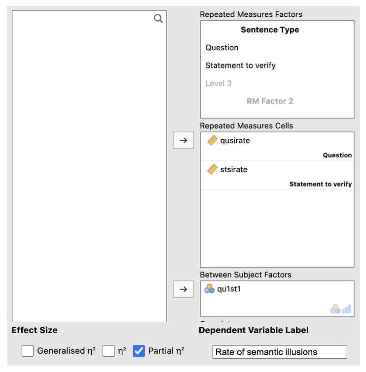
11. Go to ‘Estimated Marginal Means’. Enter the first IV in the Term 1 box. Click ‘Add New Term’. Enter the second IV into the Term 2 box. Click ‘Add New Term’. Enter the IV that you want to be displayed on the horizontal axis first in the Term 3 box (if one of your IVs is about time, e.g. ‘before’ and ‘after’ conditions, put this on the horizontal axis, e.g. in this example, it makes sense to have presentation order (qu1st1) on the horizontal axis). Enter the IV you want to be displayed as separate lines second in the box Term 3 box. Change the error bars to ‘Standard Error’. Check the box next to ‘Marginal means plots’ and ‘Marginal means tables’.

12. Go to ‘Post Hoc Tests’. Put the interaction into the box on the right. Select ‘Bonferroni’ from the Correction list.

Jamovi Output: 2x2 repeated measures ANOVA

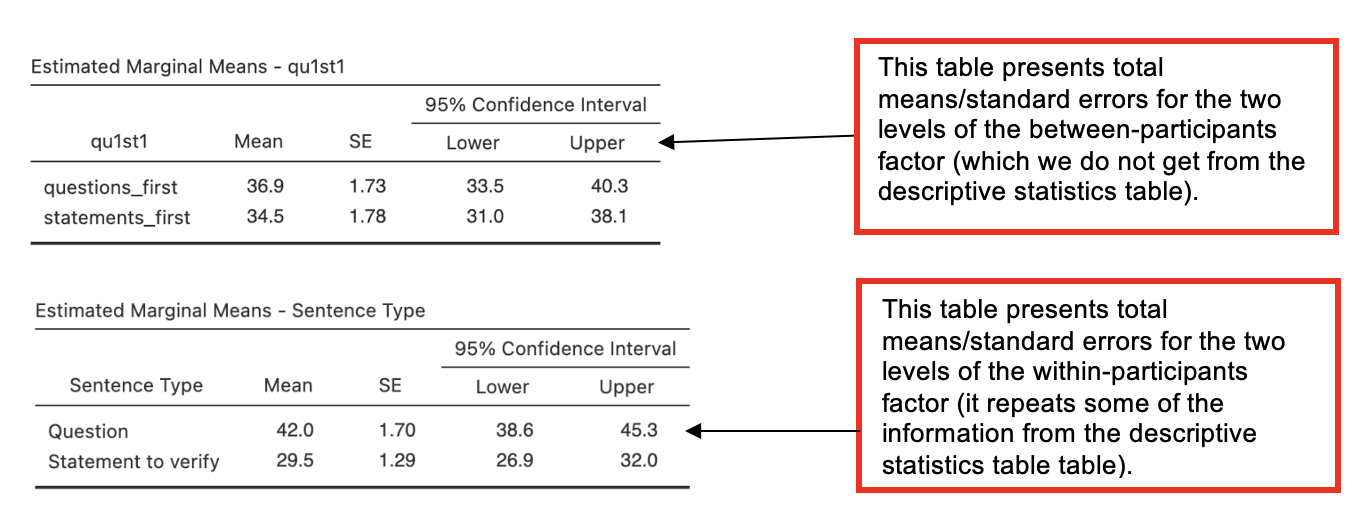
Estimated Marginal Means tables on the Jamovi output

From the next part of the output, only the most relevant tables are reproduced here: the estimated marginal means for presentation order and for sentence type.

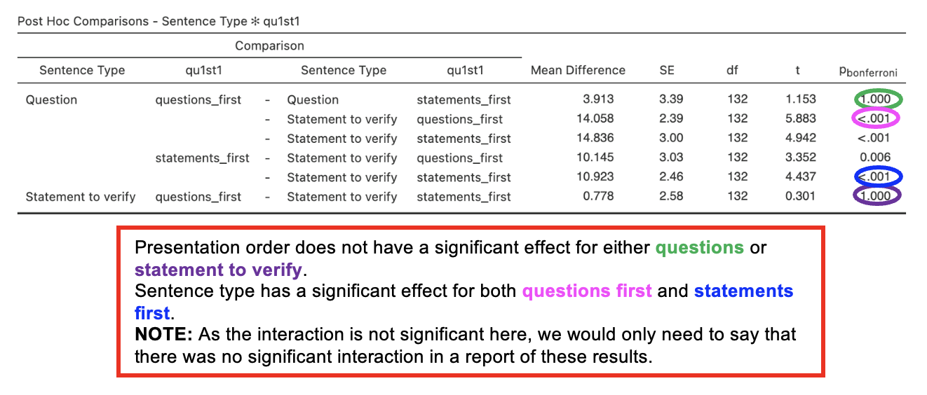
Post Hoc Comparison Tables

Interaction Plot

NoteNote - including charts

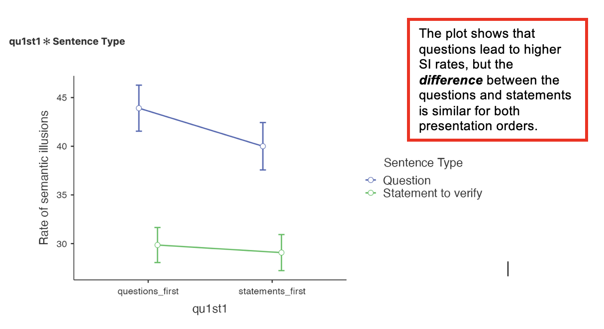
We do not usually include an interaction plot, unless the interaction is significant, and then we tend to use bar charts instead of line charts as in the Jamovi output.

Writing up 2x2 mixed ANOVAs

Tip2x2 mixed ANOVA Write Up

Fill in the blanks

(Any data preparation, e.g. how the response times were calculated or how the data were trimmed or if and how many outliers were removed, should be presented in the section of the method about data preparation and data analysis.)

In a report, an ANOVA results section could look like this:

Results (Report values to 3 d.p.)

The rate of semantic illusions for each condition was analysed using a mixed ANOVA with one within-participants factor of sentence type (question vs. statement) and one between-participants factor of presentation order (questions first vs. statements first).

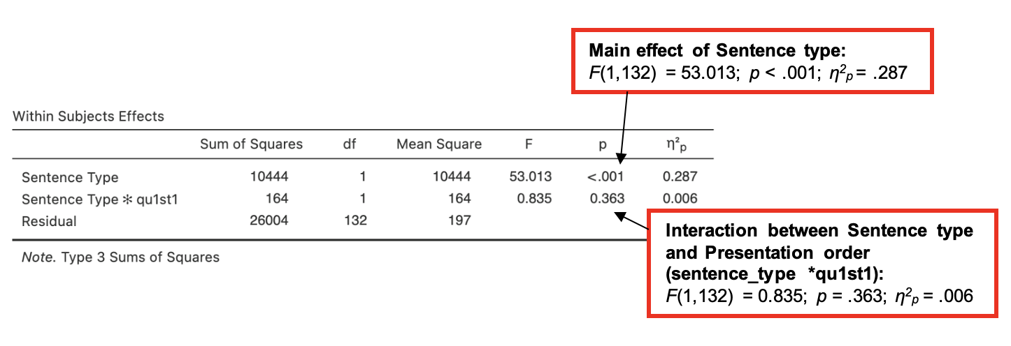
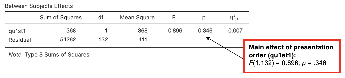
There was a significant effect of sentence type on semantic illusion rate, F() = 53.013, p < .001, η²p = , but not for the presentation order, F (1, 132) = , p = .346, or for the interaction between sentence type and presentation order, F(1, 132) = 0.835, p = .*

As predicted, the results showed that more semantic illusions occurred when the sentence was a question than when the sentence was a statement. The presentation order did not have any influence on semantic illusion rate. See Table 1 for means and standard deviations.

*Here partial eta squared is only reported for the significant effects in the analysis

Table 1. Mean semantic illusion rates (%) for questions compared to statements in both presentation orders (standard deviation in parentheses).

Presentation order	Sentence Type
	Questions	Statements
Questions first	43.9 ()	29.9 (17.1)
Statements first	(19.0)	29.1 ()

(Report values to 1 d.p.)